Shape layers
Shape layers display data such as detailed geographic boundaries and regional information. The following shape layers are supported:
In addition to shape layers, you can also define:
- Points layers – These layers display locations on the map, such as sites and customers. The sites can be from input tables or output tables. For each point layer, you control the shape, color and size of the icons that represent the sites.
- Connections layers – These layers display the flows from one location to another. They are based on flows from output tables. For each connection layer, you control the line type and color of the lines that represent the flows.
To learn more about maps, refer to:
Shaded area map
Shaded area maps (also called choropleth maps) are thematic maps in which areas are shaded or patterned based on the value of a variable being displayed on the map. For example, in Supply Chain Guru X, you may want to show a state or 3-digit zip code region colored by demand.
To set up a shaded area map, you add a layer called a Shaded Areas Layer. You then set properties for this layer including:
- Group Areas By – Select the geopolitical boundaries for determining the regions to be shaded.
- Data Source – Select the output table, field, and flow used as the data for determining the region shading.
- Class Breaks and Colors – Select the colors of the lowest and highest values for region shading, and the number of breaks by which to group the data values. Breaks result in buckets of equal size in terms of the column you select. The bucket size is determined by
maximum value - minimum value / number of breaks
Once you set the properties for the layer, the map is displayed with the selected regions shaded according to the values you have selected.
- Create a new map, or open an existing map.
- Click Show Layers.
- In the Layers section of the map controls, click Add. You see the Add Map Layer form.
- Click New, then select Shape Layer.
- Double-click Shaded Area Map, or select Shaded Area Map then click Add.
- Enter the Layer Name. The default name is “New Shaded Area Layer”.
- To define the data used for shading, select:
- Area to be Shaded – This is the boundary for the physical area to be shaded, such as Countries, World Provinces and US Counties.
- Data Source – Select the output table that is the source of the data.
- Source Field – Select the field from the Data Source that determines the actual shading.
If the Data Source is a flows table, you will also select where the data aggregation is determined:
- at Destination – The data for the Source Field is aggregated based on the destination location for the flow.
- at Source – The data for the Source Field is aggregated based on the source location for the flow.
- To define the actual shading, select:
- Number of Breaks – Select the number of value ranges to include when shading the map. The values from the output field are divided into this set of ranges, and regions are shaded based on this value.
- Start Color – Select the color to use for the first (lowest) range in the set of breaks. Colors are graded for intermediate ranges from the start to the end colors. Click the edit icon
 to control the fill color and opacity of the start color.
 - End Color – Select the color to use for the last (highest) range in the set of breaks. Colors will be graded for intermediate ranges from the start to the end colors. Click the edit icon
 to control the fill color and opacity of the end color.
- Click Add.
Shape file
These layers contain assorted shapes, such as additional geopolitical areas that are not part of the mathematical model, but are helpful for map visualization. If selected, the layer displays the data from a specific .shp shape file located on the computer.
For the Supply Chain Guru X map, shape files must be use EPSG:4326 as the coordinate system parameter. The WGS 1984 projection will not work with Supply Chain Guru X, since ESRI is not part of the Supply Chain Guru X deployment. Note that shapefiles created with WGS 1984 can be displayed with Supply Chain Guru 8.x, since that application is deployed with ESRI.
You can use the QGIS application to set the coordinate system of your shapefile to EPSG:4326. QGIS is a cross-platform free and open source GIS application available for download from qgis.org.
- Install and run QGIS Desktop.
- Click the Add Vector Layer button in the left navigation panel.
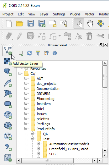
- Click Browse and navigate to your .shp file, then click Open. Your shapefile layer is displayed on the map.
- In the Layers Panel, right click on the layer you imported and select Save As...

- Click Browse and select the location for your file.
- Click the globe button at the right of the CRS setting.
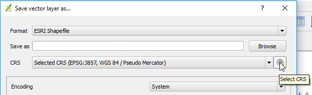
- Select "EPSG:4326" as the coordinate system. You can type in the Filter box to locate the entry. This is displayed as "(EPSG:4326, WGS 84)".
- Click OK. The saved shapefile can now be used in Supply Chain Guru X.
- Create a new map, or open an existing map.
- Click Show Layers.
- In the Layers section of the map controls, click Add. You see the Add Map Layer form.
- Click New Shape Layer.
- Double-click Shape File, or select Shape File then click Add.
- Navigate to the folder with the .shp file you want to use. Select the .shp file, then click Open.
- Enter the Map Layer Name. The default name is “New Shape Layer”.
- Optionally edit the display settings for:
- Fill – Use the controls to set the fill color and opacity.
- Border - Use the controls to set the border color, opacity and width.
- Click Add.
For map layers defined using shape files, if the shape file is not available (renamed, deleted, etc.) when the map is opened, you are prompted with a warning and the affected layer is removed. You can then discard changes to the map and replace the shape file. When you next open the map, the shape file layer will be displayed.
Service area map
The goal of service area maps is to allow you to visualize coverage (service) for a network. For example, you can use service areas to determine:
- Are all my customers within X miles?
- How many of my customers can I serve within 6, 8 or 12 hours?
Service areas can be based on straight line plus circuity distances, or using an isoline provider that is based on actual road networks, speed and bodies of water. They are calculated based on Sites, Customers or Greenfield Summary Sites (Lat/Long or Closest City) that you select.
You can calculate the service areas by either distance or time:
- Distance – You select the distance unit, then specify one or more distances, each of which is defined as a service band. If you are using an isoline provider, such as PTV XServer Internet, this is the actual road distance. If you are using Straight Line Plus Circuity as the Distance Provider, the Transportation Circuity Factor from Model Settings is added to the calculated distance when generating the bands. The band distance is calculated as:
straight line distance / (1 + Transportation Circuity Factor/100)
A positive Transportation Circuity Factor will result in a smaller band distance, while a negative Transportation Circuity Factor will result in a larger band distance.
- Time – You select the time unit, then specify one or more lengths of time. If you are using an isoline provider, such as PTV XServer Internet, this is the actual travel time. If you are using Straight Line Plus Circuity as the Distance Provider, the Default Transport Speed from Model Settings is used to determined the distance per time unit for each of the bands.
Service area map definitions are written to the ServiceAreaMap folder in the folder where your model is located.
- Create a new map, or open an existing map.
- Click Show Layers.
- In the Layers section of the map controls, click Add. You see the Add Map Layer form.
- Click New Shape Layer.
- Double-click Service Area Map, or select Service Area Map then click Add. You see the Service Area Configuration page.
- Enter a Layer Name. The default name is “New Service Area Map”.
- Select an Isoline Provider. Straight Line Plus Circuity is included. Additional providers are available if you have valid account keys populated in Application Settings > Geodata:
- HERE (not currently supported as an isoline provider)
- PTV XServer Internet
- Select a Source Table. This can be one of Sites, Customers, Greenfield Summary Sites (Lat/Long) or Greenfield Summary Sites (Closest City).
- Select one of more Locations from the Source Table. Use the Select All option to select/de-select all available locations.
You can optionally apply criteria to filter Locations from the source table.The maximum number of locations you can select for each service area map layer is 20. - Select the Service Area Basis. The default is Time-Hour. This is either a distance-unit or time-unit:
- Distance – Select a distance-unit combination, such as Distance-Mile. You specify one or more bands in terms of the selected distance unit of measure. By default, 3 color bands are created, with distances of 100, 200 and 300.
- Time – Select a time-unit combination, such as Time-Hour. You specify one or more bands in terms of travel time in the selected time unit of measure. By default, 3 color bands are created, with times of 1, 2 and 3. The Default Transport Speed in Model Settings is used to calculate the distance that can be traveled in the allowed time.
- If desired add, edit or delete color bands:
- Click Add to add another color band. By default, the new band has a Maximum Value greater than the previous band. It is calculated as the size of the previous band plus the difference between the previous two bands. For example, if you have bands of 50, 100 and 175, the next band size defaults to 250.
- Click the edit icon to control the fill color and opacity for the band.
- Edit the Maximum Value for the band. The value must be less than the subsequent band in the service area map definition.
- Click the delete icon to remove an existing band if required.
- Click Add. The service area map definition is displayed. If the definition was created with straight line plus circuity, the bands are basically circular. If the definition uses one of the other isoline providers, you see bands based on actual road networks.
PTV XInternet Server has a limit of 2 minutes for generating a service area map layer.
- Open the map with the service area map definition and click Show Layers.
- Click the edit icon for the service area map layer you want to edit.
- If desired change the Layer Name for the service area map layer.
- If desired, click the edit icon for the color band color you want to edit. You can update the fill color and opacity for the band.
- Click Save.
Last modified: Wednesday May 15, 2024