Applying and analyzing your demand model
Use the Demand Modeling tab on the workbench to choose one or more time series definitions and apply other criteria and forecasting options for analysis of your demand model.
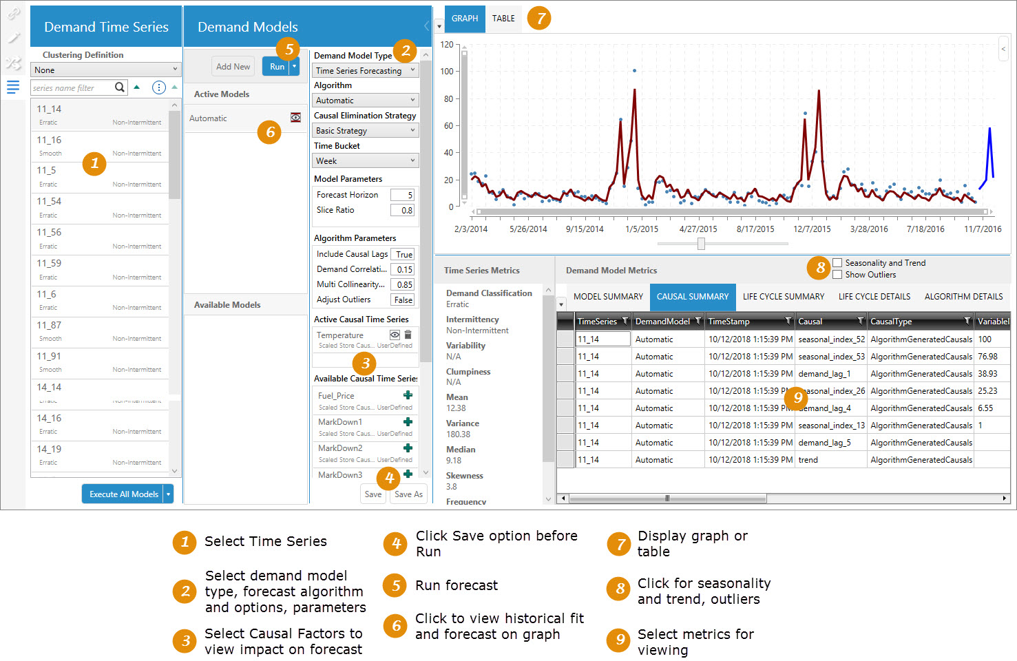
This tab allows you to explore your demand time series by creating multiple demand models that provide insight into the factors that affect the demand such as:
You can apply causal factors and create “what if” demand scenarios to enable more accurate demand prediction.
This area lists each demand time series in the model, based on the Group By Fields chosen on the Definition tab. Each time series is one group; for example, if you group by department, a time series is created for each department.
- For each demand time series, the demand classification and intermittency is also displayed; however, if Generate Time Series Only has been selected on the Definition tab, the demand classification is displayed as To be determined.
- If you have enabled the Viewer icon
 for a demand model, you can select a demand time series to quickly display the model data based on that time series in graphical or tabular format. The model data includes the run statistics for the time series.
 - If demand clusters have been defined, you can also display the cluster definitions here and then view the time series in that cluster.
Select multiple time series definitions or clusters
Several methods are available for selecting multiple demand time series and clusters.
- Ctrl + click - Use to select any combination of clusters and demand time series in the list.
- Shift + click - Use to select a group of contiguous clusters or demand time series in the list. If a cluster is not expanded, the demand time series within that cluster will not be selected.
- Ctrl + A - Once any demand time series has been selected, use to select all demand time series and clusters visible in the Demand Time Series pane. If a cluster is expanded, the demand time series within that cluster is also selected.
Note the following:
- If a demand time series or cluster is selected, but is no longer visible due to filtering (using the Filter search box, changing the demand classification categories to display, or selecting a different clustering definition), that item is not included in the selection.
- If you select more than one demand time series, or no time series are selected, the graph, table, and everything in the Demand Models pane except the Available Models list is disabled.
Execute Models
Use the options here to quickly execute all your automatic and/or user-defined models. The following execution options are available:
- Execute All Models - executes all automatic and user-defined models in Active Models
- Execute Automatic Models - executes only automatic models in Active Models
- Execute User Defined Models - executes only user-defined models in Active Models
This area is used to create, define, and execute specific demand models.
Model selection and execution
The left side of the Demand Models pane allows you to add new models, and execute selected models on specific time series.
- The Add New button creates a new active demand model, using default settings that can then be customized as needed.
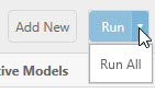
- The Run button executes the currently selected model or, optionally using the selector arrow, executes all models currently in the Active Models pane.
- Active Models are those models that can be run. By default, the Automatic model is included here. When you create a new model, it is added to this list. Initially, the model is configured with default settings and can be run immediately if desired. Once any changes are made to the model, it is moved to Available Models when the changes are saved.
- Available Models are those models that have been defined and can be applied to your time series. At any time, any of these models can be applied to one or more demand time series. Once a model has been associated with any time series, it is then listed in Active Models and is ready to be run. To add a model to the Active Models list, click the Add icon
 next to the model name.
Refer to Apply models to time series for information on how to associate models with selected time series.
Model definition
On the right side of the Demand Models pane, the model details section provides a set of criteria for defining the more unique characteristics of a selected active demand model. Several algorithm options in this area are used to choose a forecasting algorithm and specify the settings to use when running the algorithm.
- Demand Model Type - the following types can be selected -
- Time Series Forecasting - This model type predicts over a period of time for time series that may or may not have a particular pattern. It is used for both short-term and long-term predictions. Models can vary in complexity from simple rule-type models (or judgmental) to sophisticated analytical models. The Time Series Forecasting model is helpful for both short-term operational and long-term strategic plans.
For more information on this demand model type, refer to Demand forecasting.
- Life Cycle - This model type is used to generate predictions over a period of time for time series that follow a particular pattern. It is usually employed for long-term predictions by using an analytical model that performs rigid prediction estimates. The Life Cycle model is helpful for long term strategic plans.
For more information on this demand model type, refer to Life cycle modeling.
- Time Series Forecasting - This model type predicts over a period of time for time series that may or may not have a particular pattern. It is used for both short-term and long-term predictions. Models can vary in complexity from simple rule-type models (or judgmental) to sophisticated analytical models. The Time Series Forecasting model is helpful for both short-term operational and long-term strategic plans.
- Algorithm - the type of forecast algorithm to be used when running the model.
For Time Series Forecasting models, the following algorithms are available -
- Automatic - The SVM Linear, Simple Moving Average, Exponential Smoothing, and Intermittent algorithms are run in a tournament mode. The best algorithm is selected based on its performance on the test data (out-of-sample RMSE).
- Automatic Plus - The top three time series forecasting algorithms are predicted for each time series, including at least one machine learning algorithm and one classic algorithm, using historical data and RMSE with no causal data considered. Those algorithms are run using your selected error metric and causal data.
- Ensemble - When this choice is selected, all available time series forecasting algorithms are run in a tournament mode to produce a weighted average based on their respective out-of-sample RMSE values. Unlike the Tournament algorithm, you cannot add to or remove from the list of algorithms run.
- Tournament - When this choice is selected, all available time series forecasting algorithms are run in a tournament mode. The algorithm that generates the lowest out-of-sample RMSE value is selected for predicting over the forecast horizon. You can also choose to add or remove specific algorithms to/from the tournament.
- Arima - Uses a linear regression model of lags and moving average terms. Differencing is performed to make a time series stationary.
If a time series is non-stationary, the Arima algorithm takes differences between consecutive values of the time series to make a new time series. Taking such differences will make a time series stationary.
- Auto Arima - Similar to the Arima algorithm, except that all parameters are optimized by the algorithm.
- Arima X - Similar to the Auto Arima algorithm, plus support of causal data.
- Exponential Smoothing - Uses the weighted average of past observations, with weights decreasing exponentially. Instead of applying equal weight to previous data points, the highest weight is given to the most recent demand point, with progressively less weight given earlier (farther back) in the demand history. In addition to lags (past observations), this algorithm can also accommodate trend and seasonality factors in the data.
- Intermittent - Used when the demand itself is intermittent, with points in the time series when no demand is observed (value = 0). As a parameter of the Intermittent algorithm, one of 3 methods can be used: SBA (Syntetos Boylan Approximation), SBJ (Shale-Boylan-Johnston), or Croston’s Method. The default parameter value of Auto selects one of the 3 methods (Simple Exponential Smoothing, SBA and Croston’s Method) based on values of inter-demand interval mean and squared non-zero demand coefficient of variation. Valid parameter values are auto, croston, sba, or sbj.
Refer to Intermittent demand forecasting for more information on the Intermittent algorithm.
- Naïve Forecasting - This simple type of time series forecasting algorithm chooses the most recent value as the next prediction. For example, if yesterday’s ice cream sale was $960, Naïve Forecasting will predict today’s ice cream sale as $960. This algorithm is used when the time series data is quite random and does not exist in any seasonality or other recognizable patterns in data. Naïve Forecasting is generally used for benchmarking to assess the effectiveness of other, more sophisticated, algorithms.
- Simple Moving Average - Uses the unweighted mean of the last k observations in a time series, where k is a parameter. The prediction at time t, xt is calculated as -

The value of k depends on the data. If more recent values are affecting the current demand, then the value of k should be small; conversely, if the data is fluctuating considerably, then the value of k should be larger.
- Model Averaged Neural Network - Attempts to mimic the working of the human brain by building a neural network, in which basic neuron/node/units are connected to each other to form the network. The resulting multi-layered structure can be trained to estimate the ‘weights’ associated with connections between nodes of adjacent layers. Once trained, the neural network can be used to predict future demand.
- Quantile Random Forest - Builds a large number of decision trees in parallel using a sample of causal variables demand data points, and then calculates the average of predictions of all the trees.
- Stochastic Gradient Boosting - Builds a large number of decision trees sequentially. As an iterative algorithm, each new decision tree is fitted on the residuals generated by the previous tree. Output of all the trees are combined together at the end to form the final demand prediction.
- SVM Linear (Support Vector Machine) - Uses a non-linear regression model that surrounds the time series data with vectors (called support vectors) and evaluates the quality of the fit by a loss function, called epsilon loss function. It solves an optimization problem to determine the boundaries of the surrounding vectors, which minimizes this loss function.
Instead of taking a scalar product of thetas and causals, the algorithm performs a kernel trick to accomplish non-linear regression, combining multiple causals to fit a linear regression model of those combined causals in a higher dimension.
- Bass - Builds an S-shaped curve based on the effects of advertisers and customer ratings
- Gompertz - Builds an S-shaped curve based on product diffusion into the market and initial launch duration
- Logistic - Builds an S-shaped curve based on product diffusion into the market and initial launch duration
- Modified Logistic - Builds an S-shaped curve based on product diffusion into the market and expected initial demand
- Monomolecular - Models product life cycles without Launch stages, exploring expected initial demand and product diffusion into the market
- Richards - Builds an S-shaped curve based on product diffusion into the market and initial launch duration
- Triangle - Builds a cumulative S-shaped curve based only on growth and decline
- Trapezoid - Builds a cumulative S-shapted curve based only on growth, maturity, and decline
- Tournament Life Cycle - All algorithms are run in a tournament mode, and the best algorithm is selected based on AICc values (Akaike Information Criterion with correction). The algorithm that produces the lowest AICc value over the fit period is selected as the best algorithm.
- Causal Elimination Strategy - the degree to which filtering is applied by the algorithm to causal variables being considered.
When Time Series Forecasting is selected as the demand model type, selections include -
- None, for which no filtering is applied, so no causals are eliminated.
- Basic, for which two filtering methods are applied.
Correlation with Demand - If the absolute correlation coefficient value between demand and a causal fails to meet a minimum threshold, that causal is eliminated.
Multi-collinearity - If the absolute correlation coefficient value between two causals exceeds a threshold, one of the two causals is eliminated. The redundant causal variable is removed to improve efficiency and accuracy, and to minimize the chance of overfitting to the demand data.
- Advanced, for which correlation with demand and multi-collinearity are applied, and the model is fitted at each stage of the algorithm using recursive feature elimination.
When Life Cycle is selected as the demand model type, this field displays N/A.
- Time Bucket - the time increments into which data is aggregated; daily, weekly, and so on
- Model Parameters - available based on the selected algorithm and causal elimination strategy. Initially, these values are displayed as entered on the Definition tab; however, they can be overwritten here on a per model basis -
- Forecast horizon - the number of time periods in the forecast
- Slice ratio - the ratio value between 0 and 1 that represents the amount of data needed to train the forecasting model
- Key Error Metric (not available for Life Cycle models) - the error metric used for algorithm optimization when running the Automatic or Tournament algorithms. Valid entries here include RMSE, MAE, MAPE, WMAPE, ME, or MPE.
- Lead Time (not available for Life Cycle models) - the number of time bucket periods used to calculate lead time for out-of-sample MAPE.
For Life Cycle models only, these additional model parameters are available -
- Cannibalization - Indicates whether to model cannibalization between the current product and a successor product. The default is False. When set to True, these cannibalization parameters are used -
- New Product Launch Date- The launch date of the new product, expressed as YYYY-MM-DD.
- End of Life Date - The current product end of life date, expressed YYYY-MM-DD. This field is optional.
- Innovator Impact Threshold - Percentage indicating the point at which the new product cannibalizes the current product. The default is .025.
- Cannibalization Rate Adjustment - A positive value reflecting the rate at which the new product impacts the current product. The default is 1.
When you use the Cannibalization option, the table grid includes columns to separate the non-cannibalized and cannibalized results for the fitted and forecast fields, and the graph includes both the non-cannibalized curve and a cannibalized curve.
- Algorithm Parameters - determines the forecast settings by which the algorithm will be used -
- Include Causal Lags - determines whether causal lags will be calculated and used if correlated with the demand time series more closely than the actual causal
- Adjust Outliers - adjusts outlier data during model execution to improve the quality of the model fit.
- Model Names - allows you to edit the list of algorithms used in the model. For example, if Tournament is selected as the algorithm, you can add or remove algorithms from this list.
- Active Causal Time Series includes any causal time series actually being used when the demand model is run.
- Available Causal Time Series includes any other causal time series that exists and can be added to Active Causal Time Series. Use the Add icon
 next to a causal time series to add it to the active list.
 - Save and Save As preserve the current model settings, with Save As allowing you to essentially create a copy of the current model under another name. When the model is run, Demand Guru uses the last saved settings.
- Run applies the selected causal time series and generates the historic fit (represented by a continuous line running through the graph).
For Life Cycle models, the following algorithms are available -
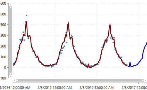
When you run the automatic model, Demand Guru detects which algorithm to use depending on the demand “signal” identified in the data, and then it selects the best model to use for more accurately predicting future demand (represented by a continuation of the line in a contrasting color on the graph).
You can collapse this section to enlarge the display of the data visualization area.
This area allows you to see how your model affects your time series data. It includes three components:
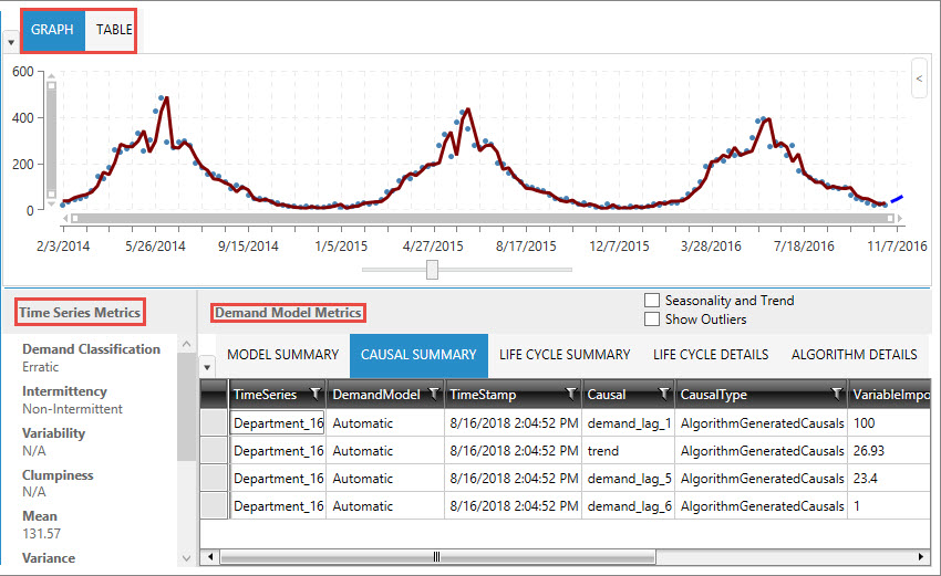
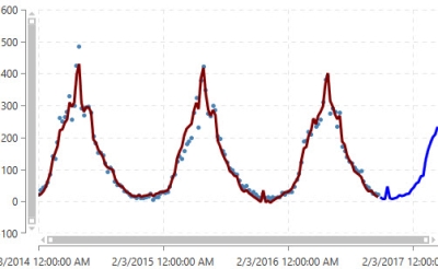
- Graph or Table display of model data.
When demand and forecast data is displayed on the graph, the historical fit is represented in the first part of a continuous line overlaying the data points, and the forecasted fit represented by the second part of the line, which is shown in a contrasting color.
- Time Series Metrics for the selected demand time series
- Demand Model Metrics for the current model
- Demand model metrics
Displays information on algorithm used, along with error metrics that help determine the accuracy of the forecast.
- Causal Summary
Lists causal variables and their ranking in the model, along with detected trends, to help determine which factors are driving demand. Based on this information, you can select one or more relevant causal time series for inclusion in the demand model graph to examine their correlation to the data.
- Life Cycle Summary
If Life Cycle was chosen as the Demand Model Type, this table highlights the various performance measures that are generated from life cycle modeling.
- Life Cycle Details
If Life Cycle was chosen as the Demand Model Type, this table consists of seven rows, one for the entire life of the product, plus one for each of the different life cycle stages.
- Life Cycle Parameters
If Life Cycle was chosen as the Demand Model Type, this table displays life cycle model parameter estimates.
- Algorithm Details
Provides information on how the algorithm was used in the model.
For Time Series Forecasting and Life Cycle demand models, the following two checkboxes are available for including addtional data in your output:
- Seasonality and Trend - Select to view seasonality effects and trend patterns in the output.
- Show Outliers - Identify outlier values in the output.
- Demand model metrics
Last modified: Thursday December 19, 2024