Demand model metrics
Demand model metrics highlight specific results from running the model.
The Model Summary table provides information on the fitted model. Note that some fields are not included for Life Cycle models.
Many of these metrics are data dependent in terms of accuracy, and their relative values alone cannot always be used as the sole basis for comparison. For example, an Out of Sample RMSE value of 400 on one time series and 10,000 on other time series does not necessarily indicate which forecast is more accurate - it depends on the mean demand.
Similarly, MAPE (Mean Absolute Percentage Error) indicates an In Sample or Out of Sample percentage error. A 10% MAPE value on one time series and 20% MAPE value on other time series does not necessarily favor the first time series in terms of accuracy - the first time series may simply exhibit more regular patterns and just be easier to forecast.
In general, the following guidelines apply:
- Lower values of these metrics indicate high accuracy.
- There should not be a big difference between the In Sample and Out of Sample values of any of these metrics. If the Out of Sample RMSE > 2 * In Sample RMSE, it means your model is overfitting. Try increasing the demand history or decreasing the number of causals used.
- Run Naïve Forecasting or Simple Moving Average algorithms. Use their In Sample and Out of Sample errors as a baseline, and compare that with the accuracy of more sophisticated (Machine Learning) algorithms to determine the level of improvement over the baseline.
Time series for which the demand profile was generated.
Name assigned by the user for the demand model. The default is Automatic.
Indicates the time at which a demand model was fit for a particular time series.
Indicates the frequency level (time bucket) of the demand time series at which a model was fitted.
Number of data points in the historical data allocated for initial training using the slice ratio.
Start date detected for each SKU.
End date detected for each SKU.
Number of data points in the historical data used as test data points.
Number of future time periods for which forecasts are generated.
Key Error Metric Selected / Key Error Metric Applied
Key Error Metric Select is the user-entered value of the error metric, while the Key Error Metric Applied is the error metric used by the algorithm. In most cases, the values of these two fields are the same. However, when values of error metrics such as MPE, MAPE, or WMAPE go to infinity, the algorithm uses the default metric RMSE as the key error metric. This generally occurs when one or more zero demand points are included in the time series.
Lead Time
The actual number of time bucket periods used to calculate lead time for out-of-sample MAPE.
Final algorithm chosen; one of the several algorithms supported by Demand Guru. For the intermittent algorithm, this field includes both the name of the algorithm and the algorithm method; for example, intermittent-auto or intermittent-croston.
For Life Cycle models, the value here is NA.
Name of the hyperparameters for the algorithm, if any, as a string. For example, Cost is a hyperparameter in the SVM Linear algorithm, with a value that can be set by a user.
For Life Cycle models, the value here is NA.
Optimal values of the hyperparameters for any algorithm.
For Life Cycle models, the value here is NA.
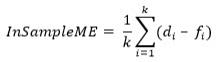
Let di represent the ith true demand point in a time series and fi denote the corresponding forecast. Then ei = di – fi is called as the forecast error.
The mean of forecast errors over the train part of the time series is the In Sample Mean Error (InSampleME).
If there are n data points in a time series, and first ‘k’ data points are in the train part, then
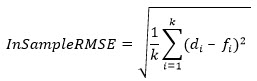
Train Root Mean Squared Error.
This value represents the square root of mean of squared error taken over the train part of the time series.
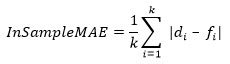
This value represents the mean of absolute differences between true demand points and forecasts over the train part of the time series.
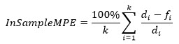
Training Mean Percentage Error.
This value represents the mean of percentage error between true demand points and forecasts over the train part of the time series.
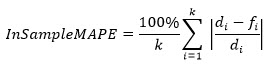
Training Mean Absolute Percentage Error.
This value represents the average of individual MAPE (Mean Absolute Percent Error) values calculated over the train part, weighted by the actual demand in each period.
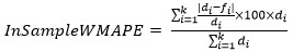
Training Weighted Mean Absolute Percentage Error.
This value represents the weighted mean of absolute values of percentage error between true demand points and forecasts over the train part of the time series.
For two periods P1 and P2, let the actual demand from those periods be D1 and D2, respectively. Also, let the forecast for the two periods be F1 and F2 respectively. If the difference between demand values and forecast values are the same for both periods (for example, if |D1 – F1| = |D2 – F2|), then the period with higher demand contributes more towards the WMAPE value. If D1 > D2, then period P1 contributes more to the error than period P2, due to the weighted average part of WMAPE formula.
Note that this field is not displayed for Life Cycle models.
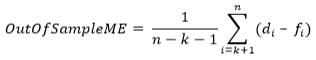
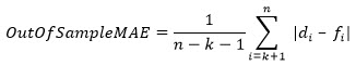
If there are n data points in a time series and first k data points are in the train part, then k+1 to n points will be in the test part. The mean of forecast error calculated over the test part of the time series is the Out of Sample Mean Error.
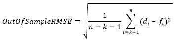
This value represents the square root of mean of squared error taken over the test part of the time series.
This value represents the mean of absolute differences between true demand points and forecasts over the test part of the time series.
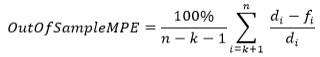
This value represents the mean of percentage error between true demand points and forecasts over the test part of the time series.
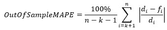
Test Mean Absolute Percentage Error.
This value represents the mean of absolute values of percentage error between true demand points and forecasts over the test part of the time series.
Test Weighted Mean Absolute Percentage Error.
This value represents the mean of absolute values of percentage error between true demand points and forecasts over the test part of the time series, weighted by the actual demand in each period.
Note that this field is not displayed for Life Cycle models.
Residuals in forecasting is a time series formed by differencing the actual demand and the fitted values obtained using the forecasting algorithm. ResidualMean is the average of residuals. ResidualMean represents the bias in the model, and an ideal model should have this average as close to zero as possible.
For Life Cycle models, this field is blank.
ResidualVariance is the variance of the residual time series in relation to the average value. When comparing different forecast algorithms, in addition to the In Sample and Out of Sample errors, comparing the variance of the residuals can also prove helpful when choosing a model.
For Life Cycle models, this field is blank.
Residual Median is the 50th percentile of the residual time series. An ideal model should have the mean and the median of residuals as close as possible.
For Life Cycle models, this field is blank.
Measures the symmetry of the residuals about their mean. An ideal model has a residual skewness close to zero.
For Life Cycle models, this field is blank.
In addition to the bias in a forecast model, an indicator of a good forecast is that the residuals are uncorrelated (independent). The LjungBox P value measures for the serial correlation in residual values. It is a hypothesis test, where the null hypothesis is that the residuals are independently distributed, while the alternate hypothesis rejects the independence claim.
Inference from the statistical test that classifies the residuals from a fitted model to be correlated with a certain level of significance. The default value of the significance level is 0.05.
For Life Cycle models, this field is blank.
Corresponding Demand Analytics version that Coupa released based on open source R.
R Version
The Causal Summary table highlights in detail the various causal variables that were utilized in fitting a machine learning model. Any causal lags detected are also included as separate rows.
Time series for which the demand profile is generated.
User-assigned name for the demand model. The default name is Automatic.
Indicates the time at which a demand model was fitted for a given time series.
Name of the causal variable. Causal lags, if enabled, are displayed here if it is determined that the lag more closely correlates with the actual causal, and are listed with a causal type of AlgorithmGeneratedCausal.
- User Defined – Causal Variable provided by the user in fitting a model.
- Promotion – Causals designated by the user as promotions.
- Trend Cloud – Causal variables pulled using the Trend Cloud Import action including, but not limited to, economic indices and weather related information.
- Algorithm Generated Causal – Causal variables automatically extracted from the time series. Patterns inherently present in the time series, such as seasonality, trend, lagged demand, and properties extracted based on calendar date, constitute such generated causals. Click here for more information related to algorithm-generated causals.
A measure indicating the relative strength of a particular causal variable in predicting the demand. A value of 100 is assigned for the strongest causal variable, while the least important causal variable is assigned a value of 1.
Classification of the causal variable depending on its strength. If a causal lag has been detected, Excluded is displayed here for the original causal.
- Insignificant – Scores between 0 and 15.
- Low Importance – Scores between 15 and 30.
- Medium Importance – Scores between 30 and 70.
- Higher Importance – Scores between 70 and 85.
- Highest Importance – Scores between 85 and 100.
Indicates whether a particular causal variable has been selected for fitting a model. If a causal lag has been detected, No is displayed here for the original causal.
Highlights the reason for dropping a causal variable. If a causal lag has been detected, an appropriate reason for the exclusion is displayed here for the original causal.
- Not Applicable – the causal variable is not dropped in the model.
- Multi Collinearity – the causal variable is better explained by another causal variable. Thus, the redundant causal variable is removed to improve efficiency, minimizing the chance of overfitting the demand.
- Lack of Correlation – the absolute value of correlation of the causal variable with the demand is extremely low. Removing such features improves efficiency and decreases the chance of over-fitting the demand.
- Recursive Feature Elimination – the causal variable is eliminated in the recursive feature elimination phase.
- Forecast Values unavailable - forecast values of the causal variable are unavailable. Thus, user-defined causal variables are ignored.
- Dropping Trend- fitted trend is dropped because of having high correlation with at least one user-defined causal variable.
A number between -1 and 1 that provides the correlation between the causal time series and the demand time series.
Classification of the causal variable based on its numeric correlation with the demand time series. Positive correlation is indicated by the suffix Positive Correlation and negative correlation is indicated by the suffix Negative Correlation. The prefix falls under one of five categories.
- Insignificant – absolute correlation with demand is between 0 and 0.15.
- Weak – absolute correlation with demand is between 0.15 and 0.30.
- Moderate – absolute correlation with demand is between 0.30 and 0.70.
- Strong – absolute correlation with demand is between 0.70 and 0.85.
- Very Strong – absolute correlation with demand is between 0.85 and 1.
Measures the degree of randomness in a causal time series and calculates how easy it is to forecast a specific time series. A lower index indicates a better ability to forecast with simple algorithms, while a higher index indicates that the time series is difficult to forecast.
Classification of Forecastability index based on its value.
- Highly Forecastable – Forecastability index value is between 0 and 0.4.
- Moderately Forecastable – Forecastability inde values is between 0.4 and 1.0.
- Somewhat Forecastable – Forecastability inde values is between 1.0 and 2.0.
- Less Forecastable – Forecastability index value is between 2.0 and 2.6.
- Random - Forecastability index value is greater than 2.6.
The Life Cycle Summary table lists the performance measures resulting from life cycle modeling.
Time series for which the demand profile is generated.
User-assigned name for the demand model. The default name is Automatic.
Indicates the time at which a demand model was fitted for a given time series.
The default name Auto is displayed when Tournament Life Cycle is selected as the algorithm. If a specific algorithm is chosen instead of the tournament algorithm, User-defined is displayed here.
Life Cycle Model
The Life Cycle algorithm ultimately used for the demand model.
This column shows the stage of the product life. Depending on the model selected and the corresponding model fit, the product could be one the following stages: Launch, Growth, Maturity, Decline, or Obsolescence.
This column shows the expected life of the product.
This column shows the total cumulative demand of a product at its maximum life.
This column shows the life of the product at which the product reaches to its maximum growth rate. Just after this point, the growth rate of the product will decline.
This column shows the total cumulative demand of the product at which the product reaches to when the product is in its maximum growth rate.
Model ID
An alphanumeric string used internally to identify the model.
The Life Cycle Details table consists of seven rows, one for the entire life of the product, plus one for each of the different life cycle stages:
- ProductLife
- Launch
- Growth
- Maturity
- HalfLife
- Decline
- Obsolescence
This table lists the start and end dates of each stage, along with its duration, based on the input data.
Time series for which the demand profile is generated.
User-assigned name for the demand model. The default name is Automatic.
Indicates the time at which a demand model was fitted for a given time series.
The stage of the life cycle, with Product Life representing the entire life cycle.
The date and time on which the stage began.
The date and time on which the stage ended.
The time length of the stage, expressed in units as selected for the Time Bucket on the Definition tab of the workbench.
An alphanumeric string used internally to identify the model.
The Life Cycle Parameters table displays life cycle model parameter estimates. Names, estimates, and standard error values of the underlying life cycle model parameters are reported in this table.
Time series for which the demand profile is generated.
User-assigned name for the demand model. The default name is Automatic.
Indicates the time at which a demand model was fitted for a given time series.
The name of the underlying life cycle model.
The name of the parameter of the underlying life cycle model.
The mean value of the parameter.
The standard error value of the parameter.
An alphanumeric string used internally to identify the model.
This output provides details related to the selected algorithm. The details are presented in text format:
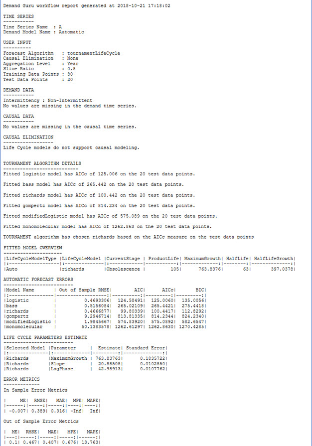
The following sections are included:
- Time Series - Standard information related to the time series.
- User Input - Standard information related to user inputs.
- Demand Data - Standard information related to demand data.
- Causal Data, Causal Elimination - These two sections present the same information for all models.
- Tournament Algorithm Details - This section appears only if the user selects Tournament Life Cycle model. It indicates the fitting quality of each enumerated life cycle model. The fitting quality is expressed as either RMSE, AIC, or AICc depending on the user selection. AICc appears as the default. Additionally, this section indicates which model is selected with the corresponding fitting quality.
- Fitted Model Overview - This table is displayed in text format and provides summary results related to the life cycle analysis of the underlying time series.
- Automatic Forecast Errors - This table is displayed in text format and provides the fitting quality of each enumerated algorithm. It appears only if the Tournament Life Cycle algorithm is selected.
- Life Cycle Parameters Estimate - This table is displayed in text format and provides names, estimates and standard error values of the underlying life cycle model parameters.
- Error Metrics - In sample and out of sample error metrics are reported for the underlying life cycle model.
Last modified: Thursday December 19, 2024