1. In the Demand Models area, click Add New.
2. When the model appears in Active Models, replace the New Model label with a meaningful name.

1. Ensure that Time Series Forecasting is selected as the Demand Model Type.
2. Use the Algorithm drop-down to select an algorithm.

   For time series forecasting models, the following choices are available in addition to the Automatic method used to establish your baseline model -

   • Ensemble - When this choice is selected, all available time series forecasting algorithms are run in a tournament mode to produce a weighted average based on their respective out-of-sample RMSE values. Unlike the Tournament algorithm, you cannot add to or remove from the list of algorithms run.
   • Tournament - When this choice is selected, all available time series forecasting algorithms are run in a tournament mode. The algorithm that generates the lowest out-of-sample RMSE value is selected for predicting over the forecast horizon. You can also choose to add or remove specific algorithms to/from the tournament.
   • Arima - Uses a linear regression model of lags and moving average terms. Differencing is performed to make a time series stationary.

     If a time series is non-stationary, the Arima algorithm takes differences between consecutive values of the time series to make a new time series. Taking such differences will make a time series stationary.

   • Auto Arima - Similar to the Arima algorithm, except that all parameters are optimized by the algorithm.
   • Arima X - Similar to the Auto Arima algorithm, plus support of causal data.
   • Exponential Smoothing - Uses the weighted average of past observations, with weights decreasing exponentially. Instead of applying equal weight to previous data points, the highest weight is given to the most recent demand point, with progressively less weight given earlier (farther back) in the demand history. In addition to lags (past observations), this algorithm can also accommodate trend and seasonality factors in the data.
   • Intermittent - Used when the demand itself is intermittent, with points in the time series when no demand is observed (value = 0). As a parameter of the Intermittent algorithm, one of 3 methods can be used: SBA (Syntetos Boylan Approximation), SBJ (Shale-Boylan-Johnston), or Croston’s Method. The default parameter value of Auto selects one of the 3 methods (Simple Exponential Smoothing, SBA and Croston’s Method) based on values of inter-demand interval mean and squared non-zero demand coefficient of variation. Valid parameter values are auto, croston, sba, or sbj.

     Refer to Intermittent demand forecasting for more information on the Intermittent algorithm.

   • Naïve Forecasting - This simple type of time series forecasting algorithm chooses the most recent value as the next prediction. For example, if yesterday’s ice cream sale was $960, Naïve Forecasting will predict today’s ice cream sale as $960. This algorithm is used when the time series data is quite random and does not exist in any seasonality or other recognizable patterns in data. Naïve Forecasting is generally used for benchmarking to assess the effectiveness of other, more sophisticated, algorithms.
   • Simple Moving Average - Uses the unweighted mean of the last k observations in a time series, where k is a parameter. The prediction at time t, xt is calculated as -

     

     The value of k depends on the data. If more recent values are affecting the current demand, then the value of k should be small; conversely, if the data is fluctuating considerably, then the value of k should be larger.

   • Model Averaged Neural Network - Attempts to mimic the working of the human brain by building a neural network, in which basic neuron/node/units are connected to each other to form the network. The resulting multi-layered structure can be trained to estimate the ‘weights’ associated with connections between nodes of adjacent layers. Once trained, the neural network can be used to predict future demand.
   • Quantile Random Forest - Builds a large number of decision trees in parallel using a sample of causal variables demand data points, and then calculates the average of predictions of all the trees.
   • Stochastic Gradient Boosting - Builds a large number of decision trees sequentially. As an iterative algorithm, each new decision tree is fitted on the residuals generated by the previous tree. Output of all the trees are combined together at the end to form the final demand prediction.
   • SVM Linear (Support Vector Machine) - Uses a non-linear regression model that surrounds the time series data with vectors (called support vectors) and evaluates the quality of the fit by a loss function, called epsilon loss function. It solves an optimization problem to determine the boundaries of the surrounding vectors, which minimizes this loss function.

     Instead of taking a scalar product of thetas and causals, the algorithm performs a kernel trick to accomplish non-linear regression, combining multiple causals to fit a linear regression model of those combined causals in a higher dimension.

   For more detailed information on these algorithms, see Time series forecasting algorithms

After choosing an algorithm for your custom model, add causal variables that you think are relevant. For example, an increase in Out of Sample RMSE indicates that the causals are negatively impacting the model; conversely, a decrease indicates that the causals are positively impacting the model.

To preserve your baseline, you create a new version of the model and make changes to the new version (similar to running an alternative scenario in Supply Chain Guru). You can then easily compare the baseline results to those of the new version and subsequent new versions.

1. In the Demand Models section of the Demand Modeling tab, click Add New to create a new version of the model.
2. With the new version selected, add all causals to the model by moving them from the list of available causals to the list of active causals.
3. Run the model using the Automatic algorithm with no causal elimination (select None for Causal Elimination).
4. Review the Model Summary, examining the out-of-sample error metrics to assess the impact of all causals on the model.

   

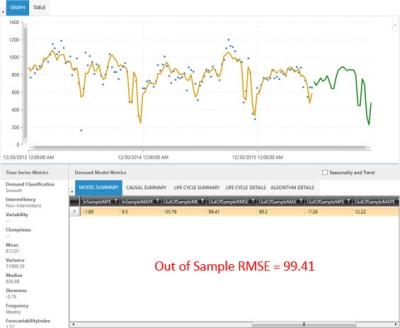
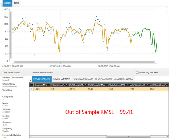
In this example:

• 5 user-defined causals are added.
• The total number of causals used is 12.
• Combined, they are hurting performance.
• The RMSE is higher than that of the baseline (99.41 > 91.42).

Model parameters are displayed as entered on the Definition tab prior to establishing your baseline model using the automatic method; however, they can be overwritten here on a per model basis.

1. For Forecast horizon, specify the number of time periods in the forecast.
2. For Slice ratio, specify a decimal value between 0 and 1 that represents the amount of data needed to train the forecasting model.
3. For Key Error Metric, indicate the error metric used for algorithm optimization. Valid entries here include RMSE, MAE, MAPE, WMAPE, ME, or MPE.
4. For Lead Time, specify the number of time bucket periods used to calculate lead time for out-of-sample MAPE.

Algorithm Parameters determine the forecast settings by which the selected algorithm will be used. The parameters listed here are available based on the selected algorithm and causal elimination strategy; however, several parameters are used by all algorithms:

• Include Causal Lags - determines whether causal lags will be calculated and used if correlated with the demand time series more closely than the actual causal
• Demand Correlation Threshold - Threshold for absolute correlation with demand between demand and a causal
• Multi Collinearity Threshold - Threshold for the absolute correlation coeffecient between two causals
• Adjust Outliers - adjusts outlier data during model execution to improve the quality of the model fit.

For information on parameters available for a specific algorithm, see Time series forecasting algorithm parameters.

Select one of the choices in Causal Elimination Strategy to determine the degree to which filtering is applied by the algorithm to eliminate causals being considered in the model:

• None - no filtering is applied, so no causals are eliminated.
• Basic - two filtering methods are applied -

  Correlation with Demand - If the absolute correlation coefficient value between demand and a causal fails to meet a minimum threshold, that causal is eliminated.

  Multi-collinearity - If the absolute correlation coefficient value between two causals exceeds a threshold, one of the two causals is eliminated. The redundant causal variable is removed to improve efficiency and accuracy, and to minimize the chance of overfitting to the demand data.

• Advanced - correlation with demand and multi-collinearity are applied, and the model is fitted at each stage of the algorithm using recursive feature elimination.