Modeling costs in transportation optimization
There are a number of costs you can apply when creating your Transportation Optimization model:
- Multi-stop route costs – Costs such as overnight charges and cost per mile. These are defined in the Rate table.
- Direct shipping cost – This cost is used for mode selection, such as with LTL and Parcel. You define this in the Direct Shipping Cost column in the Shipments table.
- Owned asset lease costs – These costs represent expenses such as maintenance and lease costs for assets. They are defined using the Fixed Asset Cost column in the Transportation Assets table.
- Segment based cost overrides – You can use these costs to represent tolls and full truckload rates. For example, you can use the Override Cost in the Transit Matrix table to override the calculated cost for specific rates. The Additive Cost in the Transit Matrix table can be used to model tolls.
- Shipment-based rates – Assign a Class Name to records in the Shipments table, then populate the Shipment-Based Rate table to define Per Unit Cost and Discount Rate values for each unique asset-source-destination-class combination. Using shipment-based rates, different costs and rates are allowed for each shipment on a route, supporting LTL aggregation (shipments with different LTL rates can be combined on a single route). See Shipment-based rates.
|
Watch this video to learn how about modeling Transportation Optimization costs. Right-click on the video and select "Open video in new tab" for a larger display: |
|
You use the Rate table to determine how the cost of your routes are calculated. You must define at least one rate record. For specific cases, Using rates as constraints can further control which routes are built.
The distance-based, time-based and stop cost fields accept either a number or a step cost name. Enter a number for a constant cost. If the cost varies with the distance, stop or time incurred, create a Step Cost Definition and associated Step Costs. For example, you can create step costs such as:
| Step Cost Name | Minimum Throughput | Cost |
| PerDistanceCost | 0 | 1.8 |
| PerDistanceCost | 300 | 1.5 |
| PerStopCost | 0 | 200 |
| PerStopCost | 3 | 225 |
By default, the rate is applied to all routes; however, you can limit the rate by asset or location:
- To limit the rate to a particular asset, select the Asset Name.
- To limit the rate by location, populate the Origin Location Group and/or Destination Location Group, then set the Rate Type in the Transportation Assets table to reflect how these rates are applied.
Calculating route costs
There are a number of cost fields within the Rate table that contribute to the total cost of the route. The basic route cost calculation is as follows:
[ Fixed Cost +
((Per Distance Cost + Surcharge Per Distance) * loaded distance +
Per Reposition Distance Cost + Surcharge Per Distance) * Reposition Distance) *
(1 + Surcharge Percentage) +
number of units * Per Unit Cost +
In-Transit Stop Count * In-Transit Stop Cost +
number of Rest Times scheduled * Fixed Rest Time Cost +
(Total Rest Time/60) * Variable Rest Time Cost +
(Drive Time/60) * Drive Time Cost +
(Non Drive Work Time/60) * Non Drive Work Time Cost +
(Wait Time/60) * Wait Time Cost +
(Break Time/60) * Break Time Cost] *
(1 – Discount Rate)
Cost to route and allocated cost
At a high level, the Cost to Route column displays what it cost to add the shipment to the route. For a given route, if Shipment A is removed, the Cost to Route for Shipment A is the difference between the original route cost and the cost without Shipment A. In this case only the delivery or pickup cost is removed from the total route cost, and the route is not reconstructed.
For example, you have a rate that charges 1.8 per distance unit and per reposition distance. The Per Stop Cost is 20 and the Per Unit Cost is 0.01. Assume you have a route with the following shipments:
| Source | Destination | Quantity |
| DC_1 | Lafayette | 1000 |
| DC_1 | Indianapolis | 750 |
| DC_1 | Dayton | 500 |
When the shipments are routed, you have the following stops:
| Stop ID | Stop Type | Site Name | Distance | Distance cost | Stop cost | Unit cost | Total |
| 0 | Equipment Start | DC_1 | |||||
| 1 | Pickup | Lafayette | 235 | 423.00 | 20.00 | 10.00 | 453.00 |
| 2 | Pickup | Indianapolis | 61 | 109.80 | 20.00 | 7.50 | 137.30 |
| 3 | Pickup | Dayton | 105 | 189.00 | 20.00 | 5.00 | 214.00 |
| 4 | Delivery | DC_1 | 190 | 342.00 | 20.00 | 342.00 | |
| Total | 1063.80 | 80.00 | 22.50 | 1166.30 | |||
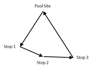
We next determine the percentage of the total load for each shipment, then prorate that to the total distance cost of the route. This is the cost based on delivering to the first and last stops on the route. For example, assume you have a route such as:
Pool Site-Stop 1-Stop 2-Stop 3-Stop 4-Pool Site
The total distance cost of the route is calculated as:
Pool Site-Stop 1-Stop 3-Pool Site
In our example, this would be:
| Stop | Distance to stop | Distance cost |
| DC_1 | 0 | 0.00 |
| Lafayette | 235 | 423.00 |
| Dayton | 150 | 270.00 |
| DC_1 | 190 | 342.00 |
| Total | 575 | 1035.00 |
The prorated cost per shipment, or “cost to route” is then calculated as:
(Shipment Qty/Total Load Qty) * Total Distance Cost of the Route
| Source | Destination | Quantity | Percentage of total load qty | “Stem” cost | |
| DC_1 | Lafayette | 1000 | 44% | 460.00 | |
| DC_1 | Indianapolis | 750 | 33% | 345.00 | |
| DC_1 | Dayton | 500 | 22% | 230.00 | |
| Total | 2250 |
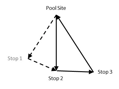
If we remove the stop for Lafayette (Stop 1), the route cost is now:
| Stop ID | Stop Type | Site Name | Distance | Distance cost | Stop cost | Unit cost | Total |
| 0 | Equipment Start | DC_1 | |||||
| 2 | Pickup | Indianapolis | 239 | 430.20 | 20.00 | 7.50 | 457.70 |
| 3 | Pickup | Dayton | 105 | 189.00 | 20.00 | 5.00 | 214.00 |
| 4 | Delivery | DC_1 | 190 | 342.00 | 20.00 | 342.00 | |
| Total | 961.20 | 60.00 | 12.50 | 1033.70 | |||
Therefore, the incremental distance cost for adding the Stop 1 is 1166.30 - 1033.70 = 132.60.
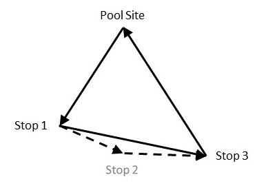
Instead, remove Stop 2:
| Stop ID | Stop Type | Site Name | Distance | Distance cost | Stop cost | Unit cost | Total |
| 0 | Equipment Start | DC_1 | |||||
| 1 | Pickup | Lafayette | 235 | 423.00 | 20.00 | 10.00 | 453.00 |
| 3 | Pickup | Dayton | 150 | 270.00 | 20.00 | 5.00 | 295.00 |
| 4 | Delivery | DC_1 | 190 | 342.00 | 20.00 | 362.00 | |
| Total | 1035.00 | 60.00 | 15.00 | 1110.00 | |||
The incremental distance cost for Stop 2 is 1166.30 - 1110.00 = 56.30.
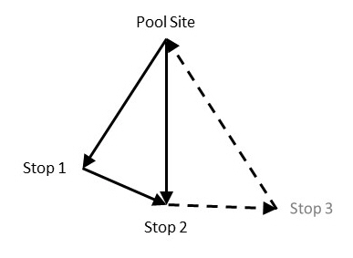
Now remove Stop 3:
| Stop ID | Stop Type | Site Name | Distance | Distance cost | Stop cost | Unit cost | Total |
| 0 | Equipment Start | DC_1 | |||||
| 1 | Pickup | Lafayette | 235 | 423.00 | 20.00 | 10.00 | 453.00 |
| 2 | Pickup | Indianapolis | 61 | 109.80 | 20.00 | 7.50 | 137.30 |
| 4 | Delivery | DC_1 | 239 | 430.20 | 430.20 | ||
| Total | 963.00 | 40.00 | 12.50 | 1020.50 | |||
The incremental distance cost for Stop 3 is 1166.30 - 1040.50 = 125.80.
Transportation Optimization generates a total computed cost that includes the incremental distance cost to route, plus the route-related cost, for each stop:
| Stop | Incremental cost | Route-related cost | Computed cost | ||
| 1 (Lafayette) | 132.60 | + | 460.00 | = | 592.60 |
| 2 (Indianapolis) | 56.30 | + | 345.00 | = | 401.30 |
| 3 (Dayton) | 125.80 | + | 230.00 | = | 355.80 |
The Allocated Cost is the computed cost multiplied by the ratio of the total route cost (1166.30) over the total computed cost (1349.70). In this case, it is the computed cost * 86%:
| Stop | Computed cost | Ratio of total route cost to total computed cost | Allocated cost |
| 1 (Lafayette) | 592.60 | 512.08 | |
| 2 (Indianapolis) | 401.30 | 86% | 346.77 |
| 3 (Dayton) | 355.80 | 307.45 | |
| Total | 1349.70 | 1166.30 |
The Allocated Cost computation method described above applies to routes with pool sites, such as those from a standard optimization problem. In the absence of a pool site, such as for routes from an interleaved optimization problem, a different method is used.
There are two types of allocated cost calculated: Distance-Based Allocated Cost and Time-Based Allocated Cost. Both cost calculations attempt to apportion the total cost of a route to each shipment. The key difference between the two allocated costs is that while the distance-based method weights each shipment’s cost by its travel distance, the time-based weights each shipment’s cost by its surface time, that is, the combination of the shipment’s travel duration and its total loading and unloading times.
Distance-Based Allocated Cost
Consider the following shipments:
| Shipment | Source | Destination | Quantity | Unit Cost |
|---|---|---|---|---|
| Ship_A | Site_1 | Site_2 | 12 | 9.00 |
| Ship_B | Site_2 | Site_3 | 1 | 0.75 |
| Ship_C | Site_2 | Site_4 | 2 | 1.50 |
| Ship_D | Site_2 | Site_5 | 1 | 0.75 |
| Ship_E | Site_2 | Site_6 | 1 | 0.75 |
| Ship_F | Site_2 | Site_7 | 1 | 0.75 |
| Ship_G | Site_2 | Site_8 | 2 | 1.50 |
| Ship_H | Site_2 | Site_9 | 1 | 0.75 |
The unit cost of each shipment is obtained by multiplying the Per Unit Cost of the route with the number of units of each shipment. The shipments are delivered by an interleaved route with the following stops:
| Stop ID | Site Name | Shipments Picked Up | Shipments Dropped Off |
|---|---|---|---|
| 0 | Site_1 | Ship_A | |
| 1 | Site_3 | Ship_B, Ship_C, Ship_D, Ship_E, Ship_F, Ship_G, Ship_H | Ship_A |
| 2 | Site_4 | Ship_B | |
| 3 | Site_5 | Ship_C | |
| 4 | Site_6 | Ship_D | |
| 5 | Site_7 | Ship_E | |
| 6 | Site_8 | Ship_F | |
| 7 | Site_9 | Ship_G | |
| 8 | Site_3 | Ship_H |
The route has a total cost of 183.64.
We first subtract the total unit costs of all shipments on the route (15.75) from the route's total cost. This gives us an adjusted total cost of 167.89. This adjusted total cost is essentially the route's total cost before factoring in the unit costs of every shipment.
We next consider each leg (the segment between each consecutive stop) of the route and its distance. We also keeps track of the shipments that are on the vehicle for each leg as follows:
| Route Leg | Origin Site | Destination Site | Leg Distance | Shipments on Vehicle |
|---|---|---|---|---|
| 1 | Site_1 | Site_2 | 78.29 | Ship_A |
| 2 | Site_2 | Site_3 | 10.13 | Ship_B, Ship_C, Ship_D, Ship_E, Ship_F, Ship_G, Ship_H |
| 3 | Site_3 | Site_4 | 1.18 | Ship_C, Ship_D, Ship_E, Ship_F, Ship_G, Ship_H |
| 4 | Site_4 | Site_5 | 0.07 | Ship_D, Ship_E, Ship_F, Ship_G, Ship_H |
| 5 | Site_5 | Site_6 | 8.26 | Ship_E, Ship_F, Ship_G, Ship_H |
| 6 | Site_6 | Site_7 | 17.15 | Ship_F, Ship_G, Ship_H |
| 7 | Site_7 | Site_8 | 41.94 | Ship_G, Ship_H |
| 8 | Site_8 | Site_9 | 7.27 | Ship_H |
We then calculate the travel distance for each shipment (the distance traveled by the vehicle with the shipment onboard). For example, shipment Ship_G is on the vehicle from legs 2 to 7, therefore its travel distance is the sum of the distances of legs 2 to 7 which is 78.73.
This distance is then multiplied by the shipment quantity to produce a Weighted Distance. A fraction is then calculated by dividing each weighted distance by the sum of all weighted distances. Finally, the allocated cost per shipment is computed by multiplying the fraction by the adjusted total cost of the route (167.89), and then adding the shipment's unit cost. A summary of these computations is shown below:
| Shipment | Unit Cost | Travel Distance | Quantity | Weighted Distance | Fraction | Allocated Cost |
|---|---|---|---|---|---|---|
| Ship_A | 9.00 | 78.29 | 12 | 939.48 | 0.732 | 131.89 |
| Ship_B | 0.75 | 10.13 | 1 | 10.13 | 0.008 | 2.08 |
| Ship_C | 1.50 | 11.31 | 2 | 22.62 | 0.018 | 4.46 |
| Ship_D | 0.75 | 11.38 | 1 | 11.38 | 0.009 | 2.24 |
| Ship_E | 0.75 | 19.64 | 1 | 19.64 | 0.015 | 3.32 |
| Ship_F | 0.75 | 36.79 | 1 | 36.79 | 0.029 | 5.56 |
| Ship_G | 1.50 | 78.73 | 2 | 157.46 | 0.123 | 22.10 |
| Ship_H | 0.75 | 86.00 | 1 | 86.00 | 0.067 | 12.00 |
Time-Based Allocated Cost
Consider the following shipments with their unit costs and their total loading and unloading times. In this example, the unit cost of each shipment is obtained by multiplying the Per Unit Cost of the route with the number of units of each shipment.
| Shipment | Source | Destination | Quantity | Unit Cost | Total Loading Time | Total Unloading Time |
|---|---|---|---|---|---|---|
| Ship_A | Site_1 | Site_2 | 46 | 92 | 23.0 | 23.0 |
| Ship_B | Site_1 | Site_2 | 39 | 78 | 19.5 | 19.5 |
| Ship_C | Site_1 | Site_2 | 16 | 32 | 8.0 | 8.0 |
| Ship_D | Site_1 | Site_3 | 56 | 112 | 28.0 | 28.0 |
| Ship_E | Site_1 | Site_3 | 35 | 70 | 17.5 | 17.5 |
| Ship_F | Site_1 | Site_3 | 16 | 32 | 8.0 | 8.0 |
| Ship_G | Site_1 | Site_4 | 62 | 124 | 31.0 | 31.0 |
| Ship_H | Site_1 | Site_4 | 36 | 72 | 18.0 | 18.0 |
| Ship_I | Site_1 | Site_4 | 15 | 30 | 7.5 | 7.5 |
| Ship_J | Site_1 | Site_5 | 56 | 112 | 28.0 | 28.0 |
| Ship_K | Site_1 | Site_5 | 34 | 68 | 17.0 | 17.0 |
| Ship_L | Site_1 | Site_5 | 16 | 32 | 8.0 | 8.0 |
Suppose these shipments are delivered by a route with the following stops:
| Stop ID | Site Name | Shipments Picked Up | Shipments Dropped Off |
|---|---|---|---|
| 0 | Site_1 | Ship_A, Ship_B, Ship_C, Ship_D, Ship_E, Ship_F, Ship_G, Ship_H, Ship_I, Ship_J, Ship_K, Ship_L | |
| 1 | Site_2 | Ship_A, Ship_B, Ship_C | |
| 2 | Site_3 | Ship_D, Ship_E, Ship_F | |
| 3 | Site_4 | Ship_G, Ship_H, Ship_I | |
| 4 | Site_5 | Ship_J, Ship_K, Ship_L | |
| 5 | Site_1 |
Also, suppose the route has a total cost of $2626.37. To apportion this total cost to each shipment, the total unit cost of all shipments on the route, $854, is first subtracted from the route’s total cost. This results in an adjusted total cost of $1772.37, which represents the route’s total cost before inclusion of the unit costs of every shipment.
The duration of each travel leg (i.e., the duration of the travel segment between each consecutive stop) of the route is then considered, together with the shipments that are on the vehicle for each leg.
| Route Leg | Origin Site | Destination Site | Travel Duration | Shipments on Vehicle |
|---|---|---|---|---|
| 1 | Site_1 | Site_2 | 277.30 | Ship_A, Ship_B, Ship_C, Ship_D, Ship_E, Ship_F, Ship_G, Ship_H, Ship_I, Ship_J, Ship_K, Ship_L |
| 2 | Site_2 | Site_3 | 18.21 | Ship_D, Ship_E, Ship_F, Ship_G, Ship_H, Ship_I, Ship_J, Ship_K, Ship_L |
| 3 | Site_3 | Site_4 | 63.51 | Ship_G, Ship_H, Ship_I, Ship_J, Ship_K, Ship_L |
| 4 | Site_4 | Site_5 | 38.69 | Ship_J, Ship_K, Ship_L |
| 5 | Site_5 | Site_1 | 199.60 |
The travel duration for each shipment (i.e., the travel duration of the vehicle with the shipment onboard) is then tallied from the table above. For instance, shipment Ship_K is on the vehicle from legs 1 to 4. Therefore, its travel duration is the sum of the durations of legs 1 to 4, which is 397.71. Next, the surface time of each shipment is calculated by summing its travel duration together with its total loading and unloading times, as shown below.
| Shipment | Travel Duration | Total Loading Time | Total Unloading Time | Surface Time |
|---|---|---|---|---|
| Ship_A | 277.30 | 23.0 | 23.0 | 323.30 |
| Ship_B | 277.30 | 19.5 | 19.5 | 316.30 |
| Ship_C | 277.30 | 8.0 | 8.0 | 293.30 |
| Ship_D | 295.51 | 28.0 | 28.0 | 351.51 |
| Ship_E | 295.51 | 17.5 | 17.5 | 330.51 |
| Ship_F | 295.51 | 8.0 | 8.0 | 311.51 |
| Ship_G | 359.02 | 31.0 | 31.0 | 421.02 |
| Ship_H | 359.02 | 18.0 | 18.0 | 395.02 |
| Ship_I | 359.02 | 7.5 | 7.5 | 374.02 |
| Ship_J | 397.71 | 28.0 | 28.0 | 453.71 |
| Ship_K | 397.71 | 17.0 | 17.0 | 431.71 |
| Ship_L | 397.71 | 8.0 | 8.0 | 413.71 |
A Weighted Surface Time is then calculated for each shipment by multiplying its surface time by the shipment quantity. This is followed by the computation of a fraction for each shipment, obtained by dividing each weighted surface time by the sum of all weighted surface times. Finally, the time-based allocated cost per shipment is computed by multiplying the fraction by the adjusted total cost of the route ($1772.37), and then adding the shipment’s unit cost. A summary of these computations is shown below:
| Shipment | Unit Cost | Surface Time | Quantity | Weighted Surface Time | Fraction | Time-Based Allocated Cost |
|---|---|---|---|---|---|---|
| Ship_A | 92 | 323.30 | 46 | 14871.80 | 0.092 | 255.94 |
| Ship_B | 78 | 316.30 | 39 | 12335.70 | 0.077 | 213.99 |
| Ship_C | 32 | 293.30 | 16 | 4692.80 | 0.029 | 83.73 |
| Ship_D | 112 | 351.51 | 56 | 19684.56 | 0.122 | 329.00 |
| Ship_E | 70 | 330.51 | 35 | 11567.85 | 0.072 | 197.52 |
| Ship_F | 32 | 311.51 | 16 | 4984.16 | 0.031 | 86.94 |
| Ship_G | 124 | 421.02 | 62 | 26103.24 | 0.162 | 411.76 |
| Ship_H | 72 | 395.02 | 36 | 14220.72 | 0.088 | 228.77 |
| Ship_I | 30 | 374.02 | 15 | 5610.30 | 0.035 | 91.85 |
| Ship_J | 112 | 453.71 | 56 | 25407.76 | 0.158 | 392.09 |
| Ship_K | 68 | 431.71 | 34 | 14678.14 | 0.091 | 229.81 |
| Ship_L | 32 | 413.71 | 16 | 6619.36 | 0.041 | 104.97 |
By default, the duration of breaks (short and long) that occur during a travel leg is included in the travel duration used for the allocated cost calculation. To exclude the duration of breaks from these travel durations, add the parameter ‘IncludeBreaksInTimeBasedAllocatedCost’ to the Config_TO table and set its value to ‘FALSE’.
Cost calculation notes
- Loaded distance is reflected on the Route Summary table by Total Distance – Reposition Distance. This is the distance traveled when the asset has one or more shipments loaded on it.
- Non drive work time is on-duty time that is not driving, nor waiting, nor taking short breaks. It is loading and unloading time specified using the service times.
- The various costs listed above can be defined as a single number or using a step function. If you are using step functions, the cost applied varies based on the step function definition. For example, if you define the Per Stop Cost using Step Costs:
Name Minimum Quantity Cost PerStopCost 0 0 PerStopCost 1 100 PerStopCost 5 125 CapInvest 500000 750000 The first stop is free, stops 2 through 5 are $100 per stop and stops over 5 are $125 each.
- If you specify Duty Time Cost, this value will be applied to the hours of on-duty time, including driving time, non-drive working time, wait time, and short breaks. In this case, Drive Time Cost, Non Drive Work Time Cost, Wait Time Cost, and Break Time Cost are ignored.
- If you define Max Duty Time Before Rest Time on the Transportation Assets table, you can set up Duty Time Cost as a step function to model regular and overtime rates. For example, assume you set the Max Duty Time Before Rest Time to 14 HR and the Duty Time Cost using Step Costs such as:
Name Minimum Quantity Cost DutyTime 0 40 DutyTime 8 50 Within each shift, the first 8 hours will have a rate of 40, the remaining hours (up to 6 per shift) will have a rate of 50. If Max Duty Time Before Rest Time is not specified, the rates will be applied to the aggregated duty time. The first 8 hours will have a rate of 40, then all remaining on-duty hours will have a rate of 50. If the route incurs 30 hours of on-duty time across multiple days, this means that 22 hours will have the rate of 50.
- The number of units applied to the Per Unit Cost is determined by the Unit Cost Basis. The basis will be one of quantity, weight or volume.
Shipment-based rates
Transportation Optimization supports Per Unit Cost and Discount Rate values at the route level, where each shipment on the route is assigned the same cost and rate. You can use shipment-based rates where different costs and rates are allowed for each shipment on a route. This functionality enables you to define route costing and rating with increased granularity. It also provides a way to model LTL aggregation, where shipments with different LTL rates can be combined on a single route.
To used shipment-based rates, you first assign a classification (Class Name) to the shipments, then create Per Unit Cost and Discount Rate values for each unique asset-source-destination-class combination in the Shipment-Based Rate table.
Using rates as constraints
You can use rates as constraints with the parameter UseRatesAsConstraint that is available in Config_TO and setting it to TRUE. Transportation Optimization only builds routes that have a populated rate record. Additionally, for origin based rates (Origin Dependent, Origin - Last Destination or Origin-Furthest Destination), “Origin” refers to the first pickup location in the route, even if this is different from the asset home site. For additional information, refer to Parameters supported in Config_TO.
Last modified: Wednesday May 15, 2024