Forecasting results based on previous data

The Time Series Forecasting action generates predictive data for a selected periodic frequency and duration, based on previous data from the same or another period. You can:

• Present data in a variety of ways
• Predict future results within an acceptable degree of accuracy

The aggregation of historical data into its proper time periods, along with the nature of the results to be presented, are defined in the action’s configuration.

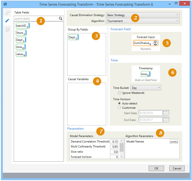
On the Configuration tab:

1. Use Table Fields to select input demand table fields.

2. Select the causal strategy and algorithm type to be used for the forecast.

3. Select the fields to be used to define groupings for time series.

4. Use Causal Variables to select causal time series variables.

5. Select the forecast input field and specify the forecast operation.

6. Define a valid timestamp field, and select time bucket and horizon options.

7. Define model parameters based on the algorithm level and type.

8. Define algorithm parameters, such as forecast data training ratio and number of time periods.

The most common application is to create time series forecasts as input to Coupa's Demand Guru.

Generate forecast results

1. Drag the Time Series Forecasting icon onto the design surface.
2. On the Connections tab , enter a Name and a Description to identify this transform, then select the input and output forecasting options.

   Input -

   • For Database Connection, select the database that contains the table with the data used for forecasting, or choose New Database Connection to establish a new connection.
   • For Input Table Name, select the table containing the demand data used for forecasting.

   Output -

   • Select the database for the forecast results, or choose New Database Connection to establish a new connection.
   • For Forecast Table Name, specify the name of the table used to tabulate the fitted and forecast values corresponding to a time series. Prediction intervals, if determined, are also tabulated.
   • For Summary Table Name, specify the name of the table used to summarize the options used to generate the fitted model, as well as behavioral and statistical information related to the model. This table includes one record for each demand time series that was forecast.
   • For Group-by Lookup Name, specify the name of the table used to map the values that were grouped on with the unique ID generated with every model run.
   • Select Generate HTML Report to create a report of the results to the output folder upon successful completion of the action.
   • Enter or select a Table Name depending on the Output Mode you choose -
     • For Create/overwrite a table, you can also choose to -
       • Add a new _autokey field to the output tables, with incremented values that make each table row unique. This is required by some database types.
       • Indicate that the output tables should be deleted after the macro or workflow has executed.

       Note that these options affect all output tables for this action.

     • For Use an existing table, indicate whether to clear the tables before execution.
3.  On the Configuration tab , choose a forecasting algorithm and specify the settings to use when running it:
   • For Causal Elimination Strategy, choose the degree to which filtering is applied by the algorithm to causal variables being considered.
     • None - no filtering is applied, so no causals are eliminated.
     • Basic Strategy - two filtering methods are applied.
       • Correlation with Demand - If the absolute correlation coefficient value between demand and a causal fails to meet a minimum threshold, that causal is eliminated.
       • Multi-collinearity - If the absolute correlation coefficient value between two causals exceeds a threshold, one of the two causals is eliminated. The redundant causal variable is removed to improve efficiency and accuracy, and to minimize the chance of overfitting to the demand data.
     • Advanced Strategy - correlation with demand and multi-collinearity are applied, and the model is fitted at each stage of the algorithm using recursive feature elimination.
   • For Algorithm, choose the type of forecast algorithm to be used when running the action. Refer to the Demand Guru Help for additional information on these algorithms. A number of the algorithms require that you have a Demand Guru license.
     • Automatic - The SVM Linear, Simple Moving Average, Simple Exponential Smoothing, and Intermittent are run in a tournament mode. The best algorithm is selected based on its performance on the test data (out-of-sample RMSE).
     • Tournament - Similar to the Automatic algorithm, three algorithms (SVM Linear, Simple Moving Average, Simple Exponential Smoothing) are run in a tournament mode. The algorithm that generates the lowest out-of-sample RMSE value is selected for predicting over the forecast horizon. Additional algorithms can be included in the tournament.
     • Arima - Uses a linear regression model of lags and moving average terms. Differencing is performed to make a time series stationary.

       If a time series is non-stationary, the Arima algorithm takes differences between consecutive values of the time series to make a new time series. Taking such differences will make a time series stationary.

     • Auto Arima - Similar to the Arima algorithm, except that all parameters are optimized by the algorithm.
     • Arima X - Similar to the Auto Arima algorithm, plus support of causal data.

       Exponential Smoothing - Uses the weighted average of past observations, with weights decreasing exponentially. Instead of applying equal weight to previous data points, the highest weight is given to the most recent demand point, with progressively less weight given earlier (farther back) in the demand history. In addition to lags (past observations), this algorithm can also accommodate trend and seasonality factors in the data.

     • Intermittent - Used when the demand itself is intermittent, with points in the time series when no demand is observed (value = 0). As a parameter of the Intermittent algorithm, one of 3 methods can be used: SBA (Syntetos Boylan Approximation), SBJ (Shale-Boylan-Johnston), or Croston’s Method. The default parameter value of Auto runs all 3 methods and selects the best one based on the out-of-sample RMSE error (error over the test dataset). Valid parameter values are auto, croston, sba, or sbj.
     • Naïve Forecasting - This simple type of time series forecasting algorithm chooses the most recent value as the next prediction. For example, if yesterday’s ice cream sale was $960, Naïve Forecasting will predict today’s ice cream sale as $960. This algorithm is used when the time series data is quite random and does not exist in any seasonality or other recognizable patterns in data. Naïve Forecasting is generally used for benchmarking to assess the effectiveness of other, more sophisticated, algorithms.
     • Simple Moving Average - Uses the unweighted mean of the last k observations in a time series, where k is a parameter. The prediction at time t, xt is calculated as -

       

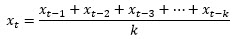
       The value of k depends on the data. If more recent values are affecting the current demand, then the value of k should be small; conversely, if the data is fluctuating considerably, then the value of k should be larger.

     • Model Averaged Neural Network - Attempts to mimic the working of the human brain by building a neural network, in which basic neuron/node/units are connected to each other to form the network. The resulting multi-layered structure can be trained to estimate the ‘weights’ associated with connections between nodes of adjacent layers. Once trained, the neural network can be used to predict future demand.
     • Quantile Random Forest - Builds a large number of decision trees in parallel using a sample of causal variables demand data points, and then calculates the average of predictions of all the trees.
     • Stochastic Gradient Boosting - Builds a large number of decision trees sequentially. As an iterative algorithm, each new decision tree is fitted on the residuals generated by the previous tree. Output of all the trees are combined together at the end to form the final demand prediction.
     • SVM Linear (Support Vector Machine) - Uses a non-linear regression model that surrounds the time series data with vectors (called support vectors) and evaluates the quality of the fit by a loss function, called epsilon loss function. It solves an optimization problem to determine the boundaries of the surrounding vectors, which minimizes this loss function.

       Instead of taking a scalar product of thetas and causals, the algorithm performs a kernel trick to accomplish non-linear regression, combining multiple causals to fit a linear regression model of those combined causals in a higher dimension space.

4. If the Performance tab is enabled in User Preferences, you can optionally change certain execution settings specific to this action. Refer to Change general preferences for additional information.

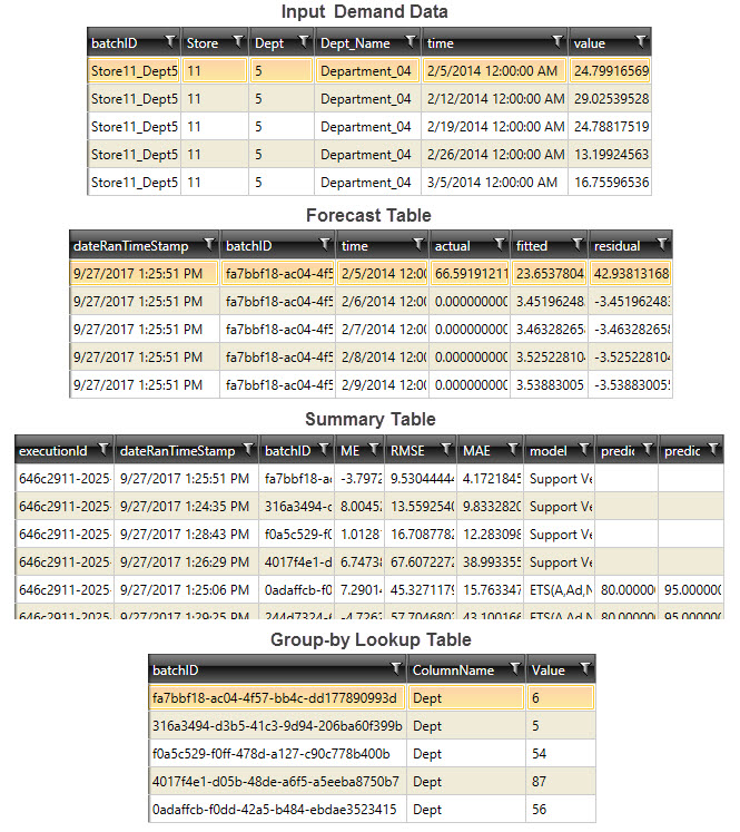
Time Series Forecasting data example

The following example shows sample demand data and the corresponding output tables generated.