Analyzing demand

The Demand Analysis action allows you to categorize each demand time series, depending on the calculated demand statistics, and produce a new table with a classification result for each product/site combination found in the input.

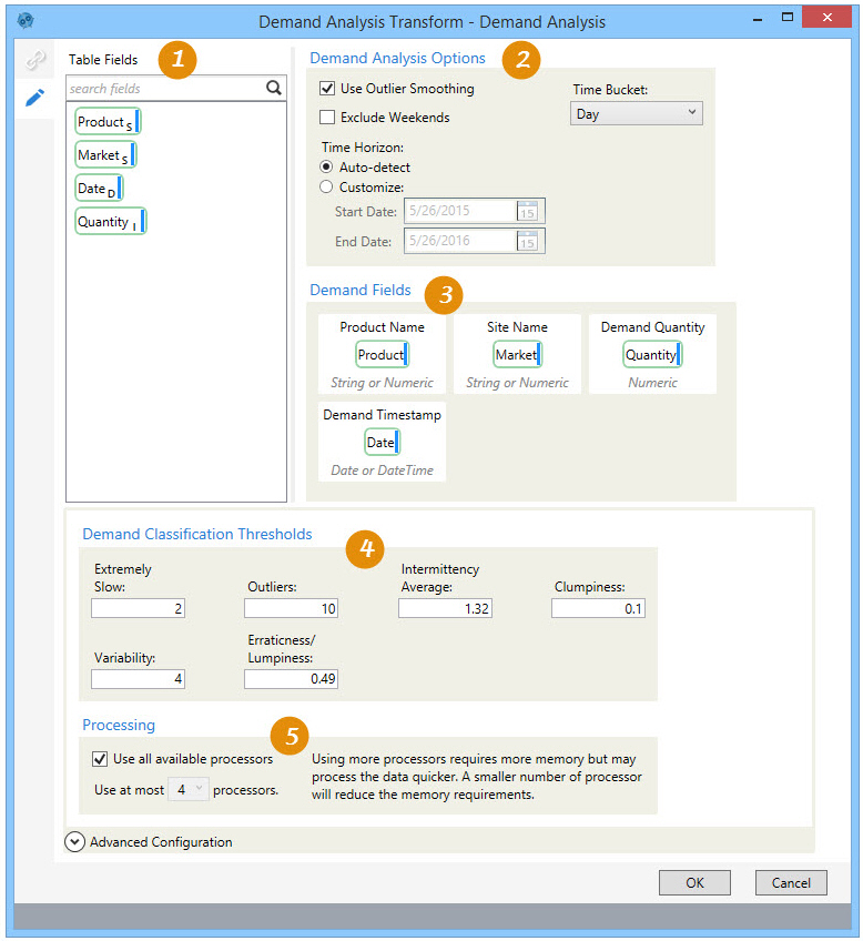
On the Configuration tab:

1. Review the Table Fields; if using multiple input tables, select the table to list the associated fields.

2. Select Demand Analysis Options, including time bucket and time horizon.

3. Drag from Table Fields to identify Demand Fields.

4. Enter thresholds for each demand classification metric.

5. Select Processing options.

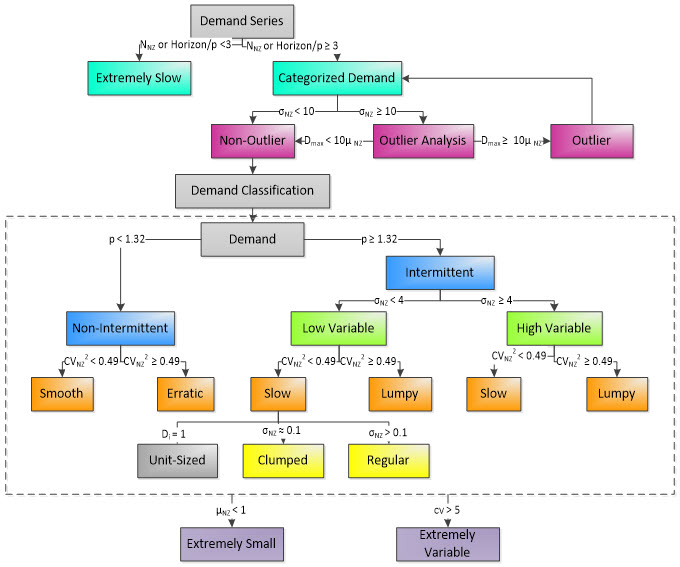
The process consists of:

• Demand characterization
  • Aggregates demand to a specified bucket – day, week or month. Supports 5-day and 7-day work weeks that let you exclude weekends from demand aggregation.
  • Summarizes demand transactions into a detailed set of statistics.
  • Identifies outliers. Outliers can be ignored or replaced with an average demand size, in which case the demand is adjusted for use in analysis.
• Demand classification
  • Classifies demand by site-product-period based on the calculated statistics.
  • Classification is based on threshold values that are user-definable.

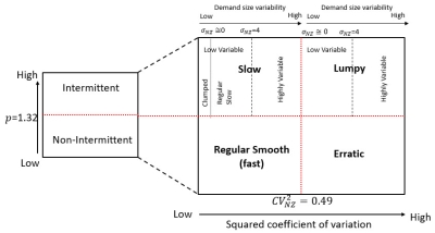
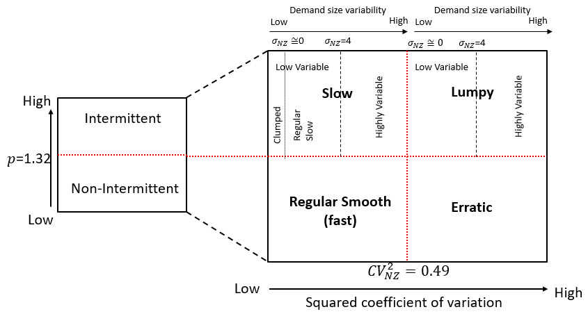
  The four main classifications include:

  • Smooth – Non-Intermittent demand with low variability compared to its mean.
  • Erratic – Non-Intermittent demand with higher variability compared to its mean.
  • Slow – Intermittent demand with low variability compared to its mean.
  • Lumpy – Intermittent demand with higher variability compared to its mean.

  Possible classifications and thresholds are shown in the following diagram:

  

  The values used for demand classification are represented by parameters defined in the following table:

  Parameter	Description
  NNZ	Non-zero demand count
  p	Mean demand intervals
  µNZ	Non-zero demand mean
  σNZ	Non-zero demand standard deviation
  CV2NZ	Squared coefficient of variation of non-zero demand. This is the variability in relation to the mean.
  Di	Aggregated demand size
  Dmax	Demand with the largest size

  The relationship between these parameters and the various classifications can be represented in this chart:

  

Possible applications include:

• Categorize Product/Customer demand as an aggregation strategy.
• Categorize the demand time series to decide on which analytical models to apply forecasting.

Run demand analysis

1. Drag the Demand Analysis icon onto the design surface.
2. On the Connections tab , enter a Name and a Description to identify this action, then specify the input delimited file and output options:

   Input -

   • For Database Connection, select the database containing the table(s) to be used as input to the analysis, or choose New Database Connection to establish a new connection to another database.
   • For Input Table Name, use the drop-down to select the table containing the demand records. Minimally, this table consists of products, sites, demand quantity, and the demand timestamp.
   • If you are including a separate table to identify additional product information, select it from the Use Product Table drop-down.
   • If you are including a separate table to identify holidays, select it from the Use Holiday Table drop-down.

   Output -

   • For Database Connection, select the database of the demand analysis table, and then enter or select a Table Name depending on the Output Mode you choose -
     • For Create/overwrite a table, enter the name of the table being created or overwritten. Using this mode, you can also choose to -
       • Add a new _autokey field to the table, with incremented values that make each table row unique. This is required by some database types.
       • Indicate that the table should be deleted after the macro or workflow has executed.
     • For Use an existing table, select the table to be used from the drop-down, and indicate whether the rows in the table should be cleared before the new data is written to the table.
3. On the Configuration tab :
   • If you have selected an optional Product Table and/or a Holiday Table on the Connections tab, use the Table Fields drop-down to control the displayed list of Table Fields and thus make it more manageable. Select a table to list its fields, or select <All Tables> to list the fields from all input tables you are using for this action.
   • For Demand Analysis Options, indicate the options by which the analysis is performed.
     • Select Use Outlier Smoothing to replace outliers with an average demand size excluding the outlier, and use the adjusted demand in the analysis. If this choice is left unselected, then outliers are detected but still included in the analysis.
     • Select Exclude Weekends to remove weekend days from the analysis.
     • Use the Time Bucket drop-down to choose the time interval by which demand is to be aggregated.
       • Day
       • Week
       • Month
     • For Time Horizon - Select Auto-detect to base the horizon on the values in the Demand Timestamp, or select Customize and indicate a Start Date and End Date.
   • In Demand Fields, drag each demand field to be used for analysis from Table Fields into the appropriate box. You must provide all of the following fields -
     • Product Name - The field containing the product for which demand is being analyzed.
     • Site Name - The field containing the site for which demand is being analyzed.
     • Demand Quantity - The field containing the site’s demand quantity for the product.
     • Demand Timestamp - The field containing the demand date or date/time.

     If you are also using a separate Product table to specify additional product information, you cannot use the same Product Name field for both.

   • If you have selected a Product Table on the Connections tab, the fields for that table are included in Table Fields and the Product Fields area is enabled. Drag the product fields from Table Fields to the appropriate box in this area. If using a product table, you must select a Product Name and at least one other product information field for this area.
     • Product Cost
     • Product Weight
     • Product Dimensions
     • Product Value
   • If you have selected a Holiday Table on the Connections tab, the fields for that table are included in Table Fields and the Holiday Fields area is enabled. Drag the appropriate date or date/time field from Table Fields to the Date box in this area.
   • Expand Advanced Configuration at the bottom of the Configuration area to set additional options -
     • Use Demand Classification Thresholds to override the default limits used for determining demand classifications.
       • Extremely Slow - Specifies at which point demand count is considered very low over the time horizon.
       • Outliers - Identifies the maximum number of outliers detected before outlier analysis is triggered.
       • Intermittency Average - Specifies the limit for average time between demand.
       • Clumpiness - Indicates when demand points are close enough together to be considered reasonably constant with almost no variability.
       • Variability - For Intermittent demand, this value determines the boundary between low variability and high variability, which indicates how much demand varies based on the Non-Zero Demand Variability.
       • Erraticness/Lumpiness - Erraticness (for Non-Intermittent demand) or Lumpiness (for Intermittent demand) specifies the threshold at which demand has a comparatively higher variability than its mean.
     • Use Processing options to set limits on the number of processors used for the analysis.
       • Use all available processors - By default, all processors that are available are used. Clear the checkbox to limit the number of processors.
       • Use at most <n> processors - If the checkbox for using all processors is cleared, the drop-down for this option is enabled, allowing you to choose the number of processors.

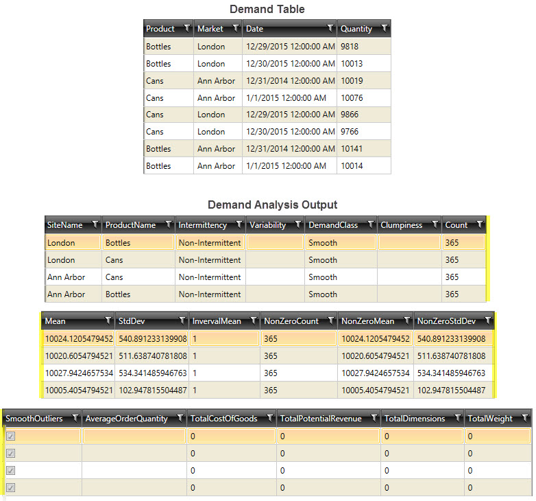
Demand Analysis data example