Simulation

Discrete event simulation is a computer-based modeling approach that represents the operation of a system as a chronological sequence of events, with the ability to incorporate variability factors as inputs to the model. Simply put, it is the representation of specific, defined events scheduled over a period of time. This can be thought of as events scheduled on a calendar, where one event's execution may lead to the scheduling of several other future events.

The following example illustrates discrete event simulation using an events calendar. The simulation maintains a list of simulation events.

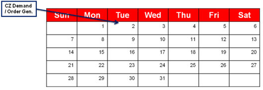
In this 31-day month calendar, various events such as demand, scheduled shipments, inventory replenishment/review, production, and delivery are scheduled.

For example, note that the first demand occurs at the customer (CZ) on the 2nd of the month.

Demand from CZ -> 10/2/09 at 4:00 pm -> Order by CZ

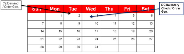
Next, an inventory review is scheduled at the distribution center (DC).

DC inventory review -> 10/3/09 at 12:00 am -> Order by DC

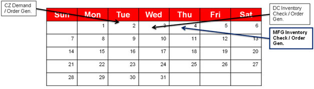
Then, a manufacturing plant (MFG) review is scheduled for order fulfillment.

MFG inventory review -> 10/4/09 at 12:00 am -> Order by MFG

After these events are observed, many events are scheduled in order to reach the final event, the shipment of product arriving at CZ.

These events are listed in order:

• Demand from CZ -> 10/2/09 at 4:00 pm -> Order by CZ
• DC inventory review -> 10/3/09 at 12:00 am -> Order by DC
• MFG inventory review -> 10/4/09 at 12:00 am -> Order by MFG
• MFG production -> 10/5/09 at 4:00 pm
• (Production order placed at the manufacturer for order fulfillment of the DC)
• Shipment leaves MFG -> 10/8/09 at 8:00 am
• (Production complete for the MFG and appropriate shipment is dispatched from the MFG to the DC)
• Shipment arrives at DC -> 10/10/09 at 2:33 pm
• (Depending on the lead time for transportation from the DC to MFG, shipment arrives at the DC 2 days later)
• Shipment leaves DC -> 10/11/09 at 8:00 am
• (DC updates its inventory position and inventory in-hand, dispatches the order to the CZ)
• Shipment arrives at CZ -> 10/11/09 at 2:22 pm

(Depending on the lead time for transportation from the DC to the CZ, shipment arrives at the customer 6 hrs and 22 min later, thereby fulfilling the final demand.)

A step-by-step simulation from the 2nd of the month (when customer order is generated) until the 18th of the month (when the order is delivered to the customer) requires individual events to occur in time. This one-by-one occurrence of events in a discrete fashion is referred to as "discrete" event simulation.

Simulation Problem Types

There are two solvers available when using Simulation. You select the solver by selecting the Problem Type when running the model in the Launch Pad.

• Classic Simulation - Classic Simulation is a discrete event simulation solver. It represents the operation of the network as a chronological sequence of events, with the ability to incorporate variability factors as inputs to the model. It is the representation of specific, defined events scheduled over a period of time.

• Simulation - This is the default Simulation solver. It is similar to Classic Simulation, but provides a faster solution and uses less RAM than the classic solver. This Simulation engine supports additional functionality not available in Classic Simulation. These features include Material requirements planning (MRP) and State Management. The new Simulation solver does not yet support all the features available with Classic Simulation (for example Process Modeling, Python Scripting, and "Ship To" constructs. Refer to Features in Simulation for the set of features supported by release in the new Simulation solver.

When using the simulation solvers, keep the following in mind:

• New features will only be added to the current (default) Simulation solver, not to Classic Simulation.

• The Simulation solver does not use input and output files in a run folder as Classic Simulation does. This is to improve performance..