Type 2 (Quantity Fill Rate)

Quantity Fill Rate is defined as the fraction of demand that is satisfied from physical inventory (available stock on shelf) on time. For Type 2 or Type 3, all stocking sites in the network must have either Replenishment Frequency or Minimum Order Quantity (MOQ) populated. If any sites do not have at least one of these values defined, the Service Definition is switched to Type1.

Coupa recommends that you set the Replenishment Frequency (RF) when using Type 2 (Quantity Fill Rate), since it is more accurate in representing the statistics than MOQ. The replenishment cycle is known as the time period between two consecutive receipts of inventory replenishment orders. The replenishment cycle is considered as the time element that is utilized to derive an approximating formula for the quantity fill rate. In this case:

For example, consider the figure below, where the system consists of a single cycle. and the shortage in the cycle is . Type 2 Service level is then calculated as:

:

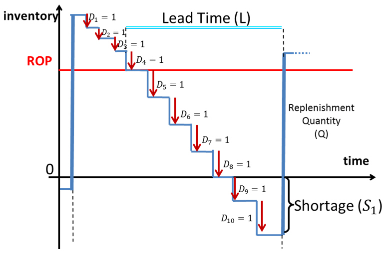
The expected demand during a cycle is often covered by a replenishment order quantity (Q). A replenishment order quantity can be optimized by an economic order quantity formula. However, in practice, it is often a challenge to determine the cost of placing an order. Therefore, one practical method to determine the size of Q is to set Q equal to the total expected demand () during a replenishment cycle (replenishment frequency, or RF).

A replenishment cycle is assumed to begin with a receipt of Q and end with the consumption of the same Q. The Type 2 basic formula in Safety Stock Optimization is:

where is the expected shortage (or backorders) at the end of a cycle. Notice that Q is a required input parameter for Type 2. For a random lead time demand variable (LTD),

The Type 2 basic formula represents a monotonically increasing function in the reorder point (R) based on the given input parameters of Q, lead time demand mean and lead time demand standard deviation. is derived for any given lead time demand distributions. For example, for a normally distributed lead time demand, for a given reorder point (R), the mean and standard deviation of lead time demand is calculated by:

where and are the standard cumulative normal distribution function and standard normal probability distribution function, respectively.

This formula works under the assumption that the demand comes in in unit sizes (i.e. size of 1). Unit size assumption also refers to another assumption that the inventory position (physical inventory - backorders + outstanding orders) is always above the reorder point. This assumption is violated along with the undershoot effect. Undershoot occurs in the case of a demand process with large demand size on a given day. The inventory position may go below the reorder point in case of a large demand size. One way to keep this assumption is to add the undershoot to the total demand during lead time. Therefore,

*corrected lead time demand mean = lead time demand mean + undershoot mean

*corrected lead time demand variance = lead time demand variance + undershoot variance

The corrected lead time demand parameters are utilized to calculate a safety stock value. Note that the corrected lead time demand parameters (mean and variance) are inclined to be larger, which causes higher safety stock values. If undershoot is ignored, then the safety stock levels will be lower too. However, the target service levels are not achieved and the actual service level will be lower than the target service level. As a result, the undershoot effect must be modeled.