Partitioning

For complex models, partitioning provides a way to break the model into smaller subproblems based on periods, products, sites, demand, customers or lanes. Modeler then solves each subproblem before determining the overall solution. The method relaxes binary variables, then fixes some binary variable values in each subproblem. This can result in better performance. Generally, the types of models that may benefit from partitioning include those with the following characteristics:

• Long solve times
• Large number of integer or binary variables due to a large defined set (periods, products, demand)
• A first integer solution is hard to find
• Feasibility is at least as important as optimality in models where a first integer solution is hard to find. While optimality is desired, a reasonable feasible solution may be acceptable in models that are extremely difficult to solve.

Partitioning works with 9 types of binary variables, such as flow and production count constraints, site open/close decisions, piecewise costs, integer lots for processes and transportation batch numbers.

When using partitioning, you select the partition type (periods, products, etc.) and the number of partitions. You control the termination of the subproblem by defining the solver time limit per subproblem and the gap percentage. See Partitioning options for more information.

When the partition size is small, each subproblem is likely to solve quickly, but there can be a large number of subproblems to solve. If the partition is too small, this can result in a long overall solve time. This approach can lean toward a more myopic decision. With larger partitions, there are less to solve, but the solution time per subproblem can be longer. This approach typically results in a more holistic decision by taking into account more discrete variables, making each subproblem closer to the original full model. As a result, it may require tuning of these parameters to find the performance sweet spot between solve time and solution quality.

When the optimality gap for subproblems is small, meaning restrictive for the corresponding partition, the overall starting solution typically starts at a better gap than if the subproblem's gap is larger. However, if subproblem gaps are too small, there may be partial solutions that are too restrictive for later subproblems to be feasible. This occurs because they are solved based on fixing variables to integer values from earlier subproblems.

Another approach for solving large Network Optimization models is decomposition. For information about when to use each approach, see Decomposition vs. Partioning.

Partitioning examples

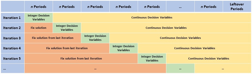
For example, you may want to partition your model based on periods. This is conventionally known as a rolling horizon solution method, not a decomposition problem. The first subproblem is solved with integer variables, while integrality is relaxed for variables corresponding to later periods.

In another example, partitioning is based on products, where partition groups are based on the percentage of total demand they cover. In this way, you can first solve an initial partition that addresses the largest percentage of total demand, while relaxing the single sourcing requirement for low volumes. These low volumes are still single sourced once the subproblem for that partition is solved. They are considered later because high volume products are solved first. The overall feasible solution may not be optimal, but it is typically close. A full feasible solution with respect to the original model is still obtained relatively quickly.