Univariate vs. Multivariate forecasting

Past demand values aid in predicting what future demand will look like. For example, suppose you are selling ice cream, with sales for the last 7 days as follows:

• $880

• $920

• $900

• $910

• $930

• $950

• $960

Based on this data, how can today’s sale be predicted?

Univariate forecasting

One way to forecast sales is to calculate the average and predict that $921.43 will be today’s sale. Another way (even simpler) is to assume that yesterday’s demand will be today’s demand as well, because $960 is the closest data point available.

The following is a plot of the sales:

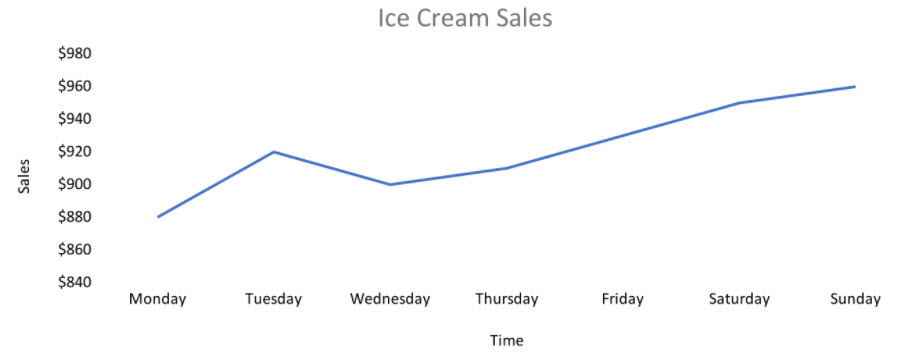
The plot might suggest an upward trend in demand, in which case the next sale should be higher than $960. However, the X-axis (time) indicates that sales are high on weekends. Because the next day is Monday, the actual sale should be much lower than $960. If last Monday’s sale ($880) is taken into consideration, a similar sale can be expected on the next Monday. Using this method, a seasonality effect has been considered.

A variety of different approaches can be applied to demand forecasting, and each approach leads to a different result. More data generally helps choose one approach over another, but nothing is guaranteed. Forecasting algorithms help find patterns in the data to yield the most accurate results possible.

In the approaches previously described, only the information from the time series was used to predict future values:

• average of last 7 days

• last value

• trend in the data

• seasonality effect

Univariate Time Series Forecasting uses only the information from the demand time series for forecasting. But what if an external factor affects your demand?

Multivariate forecasting

In the ice cream sales example, it is well known that temperature affects ice cream sales, and that ice cream sales rise when the temperature is high and drop when the temperature is lower. Should that external factor be used for forecasting?

The following is a plot that includes temperature:

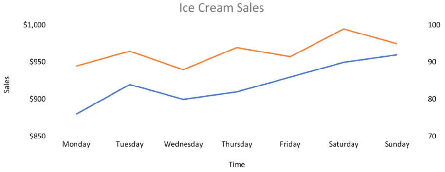
This plot indicates a high positive correlation between temperature and ice cream sales (if one increases, the other increases). Therefore, a predicted value of temperature for the next day obtained from a weather service should help us to predict the next day’s ice cream sales.

Multivariate Time Series Forecasting incorporates such external factors. This method is also referred to as causal forecasting, and in this example temperature is a causal variable that causes changes in ice cream sales.

Another example of causal forecasting is the use of marketing spend as a causal variable to forecast a company’s revenue. In this case, marketing spend is a controllable causal variable because the company can dictate how much to spend on marketing. In the ice cream sales example, the outside temperature is a non-controllable causal variable because the weather cannot be controlled. Other examples of non-controllable causal variables include macroeconomic indices, holidays, and other events or conditions occurring outside of the company.