Lead time variability in multi-echelon inventory optimization

Within multi-echelon inventory optimization (MEIO), the lead time variability is distributed among the echelons based on their coverage values. Upstream lead time variability can be pushed downstream, but not the other way around.

For example, assume the MFG fixed order time is N(3,2) days and the transportation time from the MFG to the DC is N(4,3) days.

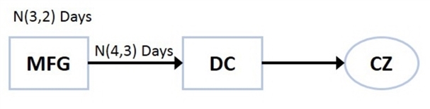
The total lead time is 3 + 4 = 7 and the total lead time variance is 22 +32 =13.

In single echelon mode, the MFG’s and DC's safety stock will cover their own lead time variability. The coverage mean and variance of the MFG are 3 and 4, respectively. The coverage mean and variance of the DC are 4 and 9, respectively. From here we can calculate the safety stock for MFG and DC.

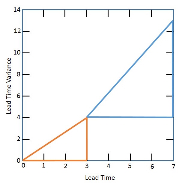
In multi-echelon mode, the MFG can push its lead time and lead time variability to the DC. But we assume that the lead time variance is evenly distributed across the network (the red line in the graphic above). If the MFG’s coverage is 2 and the DC’s coverage is 5, then their coverage variance is calculated as follows:

Coverage mean (MFG) = 2

Total lead time variance (MFG) = 2^2 = 4

Coverage variance (MFG) = Total lead time variance (MFG) * coverage mean (MFG) / Total lead time mean (MFG)

= 2^2 * 2 / 3 = 2.66667

Coverage mean (DC) = 5

Total lead time variable (DC) = 2^2 + 3^2 = 13

Coverage variance (DC) = Total lead time variance (DC) * coverage mean (DC) / Total lead time mean (DC)

= 13 x 5 / 7 = 9.29