Inventory Policies
Internal Table Name: InventoryPolicies
Use Inventory Policies to define which sites can hold products in inventory. Inventory Policies are considered unique based on the combination of Site and Product.
Evaluation of policy records depends on the use of groups and filters for the columns listed above. For more information, see Group precedence.
In Simulation, inventory policies describe when inventory is reviewed, at what level a replenishment action should occur and how/how much replenishment to take. The review is always taken against inventory position which is expected due-in + on-hand - due-out quantity.
| Due-in | On-Hand | Due Out | Inventory Position | Reorder Point | Action |
| 0 | 100 | 0 | 100 | 75 | None |
| 100 | 0 | 0 | 100 | 75 | None |
| 0 | 0 | 75 | -75 | 75 | Replenish |
| 100 | 0 | 75 | 25 | 75 | Replenish |
| 100 | 25 | 0 | 125 | 75 | None |
| 50 | 0 | 0 | 50 | 75 | Replenish |
Site
Technology: NO IO S
Table: InventoryPolicies
Internal Name: SiteName
Type: Short Text (100)
Select the site or site group for which an inventory policy is being made.
Product
Technology: NO IO S
Table: InventoryPolicies
Internal Name: ProductName
Type: Short Text (100)
Select the product or product group for which an inventory policy is being made.
Inventory Policy
Technology: S
Table: InventoryPolicies
Internal Name: InventoryPolicy
Type: Short Text (25)
Enumerated list.
Select an Inventory Policy.
| Inventory Policy | Description |
| R,Q | R,Q is a fixed replenishment point/fixed replenishment quantity inventory policy. When the inventory position falls below a certain replenishment point, R, the site will generate a replenishment order in increments, Q, of this product until the inventory position is greater than R. When using this policy, the Reorder Point column is set as the trigger level. The Reorder/Order Up To Qty column is the ‘lot’ size of units reordered. A continuous Review Period is recommended for this policy type. |
| s,S |
s,S is a minimum/maximum inventory policy. When the inventory position falls below a minimum, s, the site will generate a request for a replenishment order that will restore the on-hand inventory to a target, or maximum, number, S. When using this policy, the Reorder Point column is the minimum, or trigger level. The Reorder/Order Up To Qty column is the maximum, or the number to which the inventory level is restored. The main difference between s,S and R,Q is that the s,S takes into account exactly how far below the reorder level the inventory is when the request for replenishment is generated. The R,Q will always generate a reorder quantity in an increment of value of Reorder/Order Up To Qty until the inventory position is greater than R. The behavior of the system depends on how often inventory is checked. So, it is important to select the appropriate Review Period. |
| Demand Flow |
In Demand Flow policy, there is no strict inventory control. Instead, every order that arrives at this site for this product is not filled out of on-hand or available inventory but passed upstream to sourcing policies. When the upstream site fulfills the order and ships to this site, the fulfilled order is sent downstream. If this site is a Make site, production commences immediately for the full quantity - nothing from on-hand or available inventory is used. The Reorder Point, Reorder/Order Up To Qty and Review Period columns are not used in this policy. This policy is best used at a Make site where you do not know the inventory policies or inventory position (such as an outside vendor) but simply want the site to fulfill the order quantity received. For Simulation, available only in Classic Simulation. |
| DOS - Demand Based | Days of Supply (DOS) - Demand Based is similar to an s,S inventory policy except that the parameters for minimum and maximum levels are specified in number of days rather than product quantities. This policy computes the daily average, d, of product by looking back at the actual demand. How far back to look is given by the DOS Window field. The reorder point then equals d * Reorder Point and the reorder up to equals d * Reorder/Order Up To Qty. |
| DOS - Forecast Based |
DOS - Forecast Based is similar to an s,S inventory policy except that the parameters for minimum and maximum levels are specified in number of days rather than product quantities. This policy computes the daily average, d, of product by looking forward and using forecasted demand. How far forward to look is given by the DOS Window field. Forecast quantities must be entered into the Forecasts table for Classic Simulation and into the Site Forecasts table for Simulation. The reorder point then equals d * Reorder Point and the reorder up to equals d * Reorder/Order Up To Qty. In short, DOS-Demand establishes inventory based on what has happened; DOS-Forecast establishes inventory based on what you expect to happen. The following forecast disaggregation types are supported for New Simulation: Daily, Weekly, Weekly (5 Days), Monthly, Monthly (5 Days), Quarterly, (Quarterly 5 Days), Yearly, Yearly (5 Days). |
| R,Q - Targets |
The R,Q - Targets inventory policy allows the user to change the Reorder Point (R) and Reorder Quantity (Q) based on a period of time designated by the user (year, quarter, month, day, etc.). When using the R,Q - Targets inventory policy, the quantities and period are specified in the Forecasts input table. For Simulation, available only in Classic Simulation. |
| s,S - Targets |
The regular s,S policy is a minimum/maximum inventory policy that says that when the inventory on-hand falls below a certain minimum s, the site will request for a replenishment order that will restore the on-hand inventory to a maximum number, S. s,S - Targets inventory policy is just like the regular s,S policy except that you can specify Reorder Point (s) and Order up to Quantity (S) for certain periods. You can define the period as days, weeks, months, years, quarters etc. When using the s,S - Targets inventory policy, the quantities and period are specified in the Forecasts input table. For Simulation, available only in Classic Simulation. |
| T,S | The periodic review order up to level (T, S) policy is relatively simple and reflects real world practices to a great extent. This policy is preferred in an intermittent demand context since it facilitates the consolidation of shipments from suppliers and it is associated with the optimization of one single parameter (the order up to level). It is used to handle the Lumpy demand class, the most difficult of the classes. The periodic policy provides the convenience of regular ordering days for the stock list and for the supplier who can plan efficient routing of the delivery vehicles. |
| BaseStock |
Basestock is an (R,Q) policy with a fixed Min Replenishment Qty (Q) equal to 1. Therefore, the Reorder/Order Up To Qty field is not used. Basestock policy is useful when economies of scale in the supply system are negligible relative to other factors. For example, when each individual unit is very valuable, holding and backorder costs dominate any fixed order costs. A basestock policy is also recommended for slow-moving products where the economics of the situation rule out large batch sizes. Basestock policy is associated with the optimization of a single parameter - the reorder point. This policy is recommended with a continuous Review Period in order to improve the reaction time. |
| MRP |
This policy enables Material Requirements Planning, which is a production planning, scheduling and inventory control system use to manage manufacturing processes. MRP ensures that the correct quantity of a product is available at a point in time. The inventory position at a near future date is compared to a future forecasted demand. If the near term inventory is less than what is required for the future forecasted demand, an order is placed to cover that requirement, else no action is taken. Not available in Classic Simulation.
|
Default: s,S
Reorder Point
Technology: S
Table: InventoryPolicies
Internal Name: ReorderPoint
Type: Short Text (50)
Enter a value according to the following table:
| If Inventory Policy Is: | Reorder Point Specifies |
| R,Q or s,S | Quantity at which a replenishment order will be triggered. |
| DOS-Demand Based or DOS-Forecast Based | Number of days of supply at which a replenishment order will be triggered. |
Enter a value, then optionally select a quantity, weight or volume unit of measure, or select DOS for Days of Supply. If you do not select a unit of measure, the default Quantity Unit Of Measure from Model Settings is used.
Reorder/Order Up To Qty
Technology: S
Table: InventoryPolicies
Internal Name: ReorderQty
Type: Short Text (50)
Enter a value according to the following table:
| If Inventory Policy is: | Reorder/ Order Up To Qty Specifies: |
| R,Q | Fixed order size |
| s,S | Target quantity which inventory levels must be brought up to when a replenishment is made. |
| DOS-Demand Based or DOS-Forecast Based | Number of days of supply which inventory levels must be brought up to when replenishment order is made. |
Enter a value, then optionally select a quantity, weight or volume unit of measure, or select DOS for Days of Supply. If you do not select a unit of measure, the default Quantity Unit Of Measure from Model Settings is used.
Review Period
Technology: IO S
Table: InventoryPolicies
Internal Name: ReviewPeriod
Type: Short Text (50)
Enter how often inventory level is checked to see if a replenishment order is necessary. Enter a value, then optionally select a time unit of measure. If you do not select a unit of measure, the default Time Unit Of Measure from Model Settings is used. Options for Review Period are Hourly, Daily, Weekly, Monthly, and Continuous. Continuous means that every order that arrives will cause the inventory level at that site to be checked to see if a replenishment order is necessary.
For many supply chains, automated inventory tracking means that they continuously check the inventory level, replenishing almost the instant that the level falls below the Reorder Point. However, there are also cases where the actual behavior of the system is really better represented by a periodic review system.
For example, your Lemonade Stand always knows how much inventory is on-hand, but only wants to replenish once a day. In this case, a Review Period of “Daily” would result in product being reordered once a day, but only if needed.
The Review Period can be set to a pre-defined interval, set to one value, or assigned a schedule as well. The following table illustrates how to enter data in this field:
| Value | Examples | Parameter use |
| Interval | Continuous, Daily, Weekly | The inventory level is evaluated at each pre-defined interval. |
| Single Value |
12 HR 1 DAY |
The inventory level is evaluated every interval value (for example, every 12 hours). |
| Repeating Schedule | 1 DAY, 3 DAY, 2 DAY | The inventory level is reviewed after one day, then reviewed again 3 days after the first review, and again 2 days after the second review. The schedule is repeated upon completion. |
| Day of Week |
MON 0700, TUE 1200 wed 0930,wed 1500 Fri 1115 , TUE 1330 , Mon 0800
The following value is invalid: Tues 900,,WED 1700, |
This is used with the "Simulation" problem type only. The shipment occurs on Monday at 07:00 am and Tuesday at 12:00 pm. Notes for usage:
Not permitted:
|
Review periods themselves are dependent on the start time of Simulation. For example, assume the start time set in the Model Settings is 12:00 AM 1/1/2010, and the Review Period is set to 24 HR. The inventory level is reviewed every day at 12:00 AM. You can enter an offset in front of the Review Period to change the time the model will start reviewing. The offset is incurred only once. For example, if you want to review the inventory level every day at 4 PM, and Simulation starts at 12 AM, enter an offset of 16 hours to shift the review time to 4 PM. Then, if the Review Period is 24 HR, it checks every 24 hours from the time to which it was offset. The format for the offset is:
< "time" >
For a 16 hour offset, with a daily Review Period, you would enter: <16 HR>, 24 HR.
Default: Continuous
Forecast Name
Technology: S
Table: InventoryPolicies
Internal Name: ForecastName
Type: Short Text (100)
In this column choose the forecast you want to use for a DOS - Forecast Based inventory policy or the targets for an R,Q-Targets or s,S-Targets inventory policy. These forecasts can be specified on the Forecasts table.
Forecast Aggregation Period
Technology: S
Table: InventoryPolicies
Internal Name: ForecastAggregationPeriod
Type: Short Text (25)
One of Daily, Weekly, Monthly, Quarterly, Yearly
Select the time period at which the forecast quantities are aggregated using the records in the Site Forecasts table. This data is used when the Inventory Policy is "DOS - Forecast Based" or "MRP".
Default: Daily
Forecast Disaggregation Pattern
Technology: S
Table: InventoryPolicies
Internal Name: ForecastDisaggregationPattern
Type: Short Text (25)
One of 5 Days, 7 Days
This value determines the pattern you are using when forecasting. Select whether the forecast quantities are disaggregated based on a 5-day or 7-day week basis.
Initial Inventory
Technology: NO IO S
Table: InventoryPolicies
Internal Name: InitialInventory
Type: Short Text (50)
Enter the amount of this product that is on-hand at this site when the simulation begins running. Enter a value, then optionally select a quantity, weight or volume unit of measure. If you do not select a unit of measure, the default Quantity Unit Of Measure from Model Settings is used.
In supply chain simulation, you are starting from scratch each time. Although your model will quickly conform to a real world situation, at time zero, there will likely be differences between the model and the real world. You can counteract some of these differences by setting initial inventory levels in your model.
Safety Stock Optimization does not consider Initial Inventory.
Default: 0
Unit Inbound Cost
Technology: NO IO S
Table: InventoryPolicies
Internal Name: InboundCost
Type: Short Text (255)
Enter the activity cost of handling and moving one unit of this product from the receiving dock into inventory.
This figure contributes to inbound warehousing cost statistics in your simulation report.
Unit Inbound Cost does not include transportation costs.
Unit Inbound Cost is reflected on the following tables:
- Network Summary Optimization Output Table in the Total Inbound Warehousing Cost column.
- InterSite Flows Optimization Output Table in the Flow Inbound Warehousing Cost column. The costs are reported on a source-destination basis. You can use a filter to get an aggregated view based on Product and Destination.
Use of piecewise costs can lead to numerical issues that result in infeasibility. In this case, you may want to select the “Handle Using Logic Constraints” Network Optimization option. This option can be useful when your model contains piecewise costs that lead to binary variables and BigM constraints.
For information about using costs in multi-period models, refer to Multi-Time Period Costs and Constraints.
Fixed Inbound Shipment Cost
Technology: S
Table: InventoryPolicies
Internal Name: InboundShipmentCost
Type: Short Text (100)
Enter the activity cost of handling and moving a shipment of this product from the receiving dock into inventory. This figure contributes to inbound warehousing cost statistics in your simulation report.
Unit Outbound Cost
Technology: NO IO S
Table: InventoryPolicies
Internal Name: OutboundCost
Type: Short Text (255)
Enter the activity cost of removing one unit of this product from inventory to the shipping dock.
This figure contributes to outbound warehousing cost statistics in your simulation report.
Unit Outbound Cost does not include Transportation costs.
Unit Outbound Cost is reflected on the following tables:
- Network Summary Optimization Output Table in the Total Outbound Warehousing Cost column.
- InterSite Flows Optimization Output Table in the Flow Outbound Warehousing Cost column. The costs are reported on a source-destination basis. You can use a filter to get an aggregated view based on Product and Source.
- Customer Flows Optimization Output Table in the Flow Outbound Warehousing Cost column. These are the outbound warehousing costs facing customers. The costs are reported on a source-destination basis. You can use a filter to get an aggregated view based on Product and Source.
Use of piecewise costs can lead to numerical issues that result in infeasibility. In this case, you may want to select the “Handle Using Logic Constraints” Network Optimization option. This option can be useful when your model contains piecewise costs that lead to binary variables and BigM constraints.
For information about using costs in multi-period models, refer to Multi-Time Period Costs and Constraints.
Fixed Outbound Shipment Cost
Technology: S
Table: InventoryPolicies
Internal Name: OutboundShipmentCost
Type: Short Text (100)
Enter the activity cost of removing a shipment of this product from inventory to the shipping dock. This figure contributes to outbound warehousing cost statistics in your simulation report.
Inbound Capacity
Technology: NO
Table: InventoryPolicies
Internal Name: InboundCapacity
Type: Short Text (100)
Enter the maximum quantity of product this site is capable of accepting. You can also leave it blank to define a capacity with no maximum. Enter a value, then optionally select a quantity, weight or volume unit of measure. If you do not select a unit of measure, the default Quantity Unit Of Measure from Model Settings is used.
For information about using constraints in multi-period models, refer to Multi-Time Period Costs and Constraints.
Outbound Capacity
Technology: NO
Table: InventoryPolicies
Internal Name: OutboundCapacity
Type: Short Text (100)
Enter the maximum quantity of product this site is capable of shipping. You can also leave it blank to define a capacity with no maximum. Enter a value, then optionally select a quantity, weight or volume unit of measure. If you do not select a unit of measure, the default Quantity Unit Of Measure from Model Settings is used.
For information about using constraints in multi-period models, refer to Multi-Time Period Costs and Constraints.
Constraint Period
Technology: NO
Table: InventoryPolicies
Internal Name: ConstraintPeriod
Type: Short Text (50)
One of: Period Length, Day, Week, Month (30 day), Quarter (91 day), Year.
Choose the time period over which the Inbound Capacity and Outbound Capacity is applied.
Default: Period Length
Inventory Turns
Technology: NO
Table: InventoryPolicies
Internal Name: InventoryTurns
Type: Short Text (100)
This column allows you to specify a (piecewise) linear function from which the average inventory can be calculated during optimization.
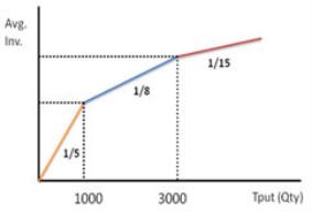
We define the following relationship between Average Inventory and Throughput:
Average Inventory = m times Throughput
Where m is the inverse of the inventory turns value.
We allow Average Inventory to be defined over multiple ranges of Throughput. The format for the relationship is a series of pairs <lower range value, turns value>.
Consider the sample graph below. Up to 1000, the Average Inventory is (1/5) * Throughput. Between 1000 and 3000, the Average Inventory is (1/8) * Throughput + 75. After 3000, the Average Inventory is (1/15) * Throughput + 250. This relationship is to be entered as <0|5><1000|8><3000|15>. In the case the relationship between Average Inventory and Throughput is simply linear, it is sufficient to input the turns value (inverse slope) of this line; for example, 5.
Unhealthy Turn Percent
Technology: NO
Table: InventoryPolicies
Internal Name: UnhealthyTurnPercent
Type: Number (Double)
Enter the percent of additional inventory that is holding space in the model beyond turn-based inventory. The value is expressed as a percentage of the turns.
Fixed Excess Stock
Technology: NO
Table: InventoryPolicies
Internal Name: FixedExcessStock
Type: Short Text (100)
Enter the additional stock held at the site that is not able to serve demand. Unless this stock can be moved (based on Excess Move Percent), it consumes space in the site to which it is assigned. Enter a value, then select a Quantity, Weight or Volume unit of measure. If you do not select a unit of measure, the default Quantity Unit Of Measure from Model Settings is used.
Excess Move Percent
Technology: NO
Table: InventoryPolicies
Internal Name: ExcessMovePercent
Type: Number (Double)
Enter the percentage of the site's Fixed Excess Stock that can be moved to a different site to free up space for standard product movements. The default of 0 means that no stock can be moved. In order for stock to move between sites, active lanes must be defined in the Transportation Policies and Site Source Policies tables to support that movement.
Inv Carrying Cost %
Technology: NO IO
Table: InventoryPolicies
Internal Name: InvCarryingCostPercentage
Type: Number (Double)
Specifies the cost percentage for holding inventory of specified product at this site during the optimization run. This percentage and the Product Value are used to calculate inventory holding costs. If the inventory carrying cost percentage is 10%, enter "10" in this column. If this value is not specified, the Inv Carrying Cost % defined in Model Settings is used. Note that a value of 0 for Inv Carrying Cost % is treated the same as a null value. In this case the Inv Carrying Cost % defined in Model Settings is used.
Inv Carrying Cost % is reflected in the Total Inv Holding Cost in the Network Summary output table.
Minimum Dwell Time
Technology: NO S
Table: InventoryPolicies
Internal Name: MinDwellTime
Type: Number (Long Integer)
Network Optimization: This column determines the minimum number of periods in which a product must stay at the site. The value must be a non-negative integer. For example, if the Min Dwell Time is set to 2, and the product is produced in Period_001, it must remain in inventory at the site for Period_001 and Period_002 before being used to fulfill demand.
Simulation: You can use the Min Dwell Time field to determine how long a product must remain at the site. The product will not be available to satisfy demand until the Min Dwell Time has been reached. These products are considered part of inventory.
You can use this feature to determine how early products can or should be pre-built, and when they should be pushed out from a site. If you are using ShipTo business logic, dwell time can be used to define cross docking. Additionally, you can use dwell time to define seasonal production methods.
Enter the Min Dwell Time as a number of days, using a non-negative integer value.
Maximum Dwell Time
Technology: NO S
Table: InventoryPolicies
Internal Name: MaxDwellTime
Type: Number (Long Integer)
Network Optimization: This column determines the maximum number of periods in which a product can stay at the site. The intent of this value is to push a product out of the site after the number of periods specified by Max Dwell Time. A common use is to limit how early products can be pre-built. The value must be a non-negative integer. A value of 0 means the product cannot be pre-built at all; it can only be produced in the same period in which it is demanded. Initial inventory is treated like it came into the system in the period before the model starts (that is, period 0). If the Max Dwell Time value in Inventory Policies is set to 1, this initial inventory can be used to fulfill demand in period 1, but not period 2, or subsequent periods. If the Max Dwell Time is set to 2, initial inventory can be used to fulfill demand in periods 1 and 2, but not 3, 4, and so on.
Simulation: You can use the Max Dwell Time to limit how long, in days, a product can remain at the site. Once this limit is reached, the product expires. At an inventory review, if the product has exceeded its Max Dwell Time at the site, it is removed from available inventory and added to the cumulative scrap output.
You can use this feature to determine how early products can or should be pre-built, and when they should be pushed out from a site. If you are using ShipTo business logic, dwell time can be used to define cross docking. Additionally, you can use dwell time to define seasonal production methods.
Enter the Max Dwell Time as a number of days, using a non-negative integer value.
Maximum Inventory
Technology: NO
Table: InventoryPolicies
Internal Name: MaxInvQty
Type: Short Text (100)
Specifies the maximum amount of specified product that this site can stock. Enter a value, then optionally select a quantity, weight or volume unit of measure. If you do not select a unit of measure, the default Quantity Unit Of Measure from Model Settings is used.
Minimum Inventory
Technology: NO
Table: InventoryPolicies
Internal Name: MinInvQty
Type: Short Text (100)
Specifies the minimum amount of specified product that this site is required to stock. Enter a value, then optionally select a quantity, weight or volume unit of measure. If you do not select a unit of measure, the default Quantity Unit Of Measure from Model Settings is used.
Safety Stock
Technology: NO
Table: InventoryPolicies
Internal Name: SafetyStock
Type: Short Text (100)
Specifies the quantity or Days of Supply that will be held in inventory. Enter a value, then optionally select a quantity, weight or volume unit of measure, or select DOS to specify Days of Supply. If you do not select a unit of measure, the default Quantity Unit Of Measure from Model Settings is used. This value can be changed by period in the Multi-Period Inventory Policies table. This column is an input for Network Optimization (and is not used in Simulation). To calculate this value, use Safety Stock Optimization.
Unit Disposal Cost
Technology: NO
Table: InventoryPolicies
Internal Name: Disposal Cost
Type: Short Text (100)
Enter the disposal cost that is incurred when the shelf life expires for this product at this site. You can control the disposal cost per period by setting a Unit Disposal Cost in the Inventory Policies Multi-Period table.
Network Optimization supports disposal cost both for products that expire based on their shelf life and those by-products that are trash (not expired)
- Expired Products – If the product reaches its shelf life before the model ends, it is an expired product. You can define a disposal cost that is incurred when the shelf life of a product expires within the model horizon. Network Optimization will determine whether it is cheaper to incur the disposal cost and get rid of the product when expired, or convert it into another product through relevant Bills Of Material before the product expires.
The Unit Disposal Cost column in the Inventory Policies and Inventory Policies Multi-Period tables enable you to set a disposal cost per product per site for each time period. You must define Inventory Policies for products that can expire, even if you are not applying a Unit Disposal Cost.
For expired products, the cost is reported in the Flow Transportation Cost field on the Customer Flows Optimization Output table, for a flow with a Customer named "Trash". The Mode is “EXPIRED PRODUCT”.
- Trashed Products – A by-product is considered trash if it has not reached its expiration date (end of shelf life) by the end of the model and if there are no Inventory Policies defined for the product. If there are Inventory Policies defined, it is assumed that the by-product should be held in inventory, rather than trashed. In this case, an inventory holding cost may be incurred.
If a by-product is to be trashed (that is, no Inventory Policies have been defined), you can define a disposal cost to be incurred for an unexpired by-product, in other words the cost to dispose of by-products created as part of your Bills Of Material. This is referred to as a “trashing cost” and applies to unused, unexpired by-product. You specify this using the “Disposal cost per unit of by-product” on the Modeling Options tab of Optimization Options.
The disposal cost for trashed products is reported in the Flow Transportation Cost column on the Customer Flows Optimization Output table, for a flow with a Customer named "Trash". The Mode is “UNUSED PRODUCT”.
Unit Storage Cost
Technology: NO S
Table: InventoryPolicies
Internal Name: InventoryCostOther
Type: Number (Float)
Enter the cost per unit of inventory per period.
Product Inventory Value
Technology: NO IO
Table: InventoryPolicies
Internal Name: ProductInventoryValue
Type: Number (Double)
Enter a monetary value for each unit of the product at the site. The Product Inventory Value column is used to calculate the inventory investment and inventory holding costs. This enables you to vary the product value at a specific site. It is incorporated in the following formula:
Inventory holding cost = Inventory Quantity * Product value * Holding Cost Percentage * Length of Time in Inventory
The Product Inventory Value in the Inventory Policies table overrides the Product Value in the Products table for both Network Optimization and Inventory Optimization. In Simulation, the Product Value in the Products table is always used.
Product Taxable Value
Technology: NO
Table: InventoryPolicies
Internal Name: ProductTaxableValue
Type: Number (Double)
When you define records in support of taxes and duties, the Product Taxable Value is used to determine the product value for taxation purposes in some cases. You can set up Tax And Duty Regions, each of which has a Source and Destination. When the locations used for the Source and Destination are sites (not customers), the Product Taxable Value from the Inventory Policies table is used to determine the product value. You can also define period-specific product values in the Inventory Policies Multi-Period Unit Taxable Value column. This value is overridden by values populated in the Taxable Value Overrides table. If this value is not populated and you have no Taxable Value Overrides defined, the Unit Value from the Products table is used.
Stocking Site
Technology: NO IO
Table: InventoryPolicies
Internal Name: StockingSite
Type: Bit
One of Yes, No. (Actual database values are 1,0.)
Use this field to determine if a site can hold safety or prebuilt stock. The default value is "Yes". This setting is used in Network Optimization and Safety Stock Optimization. In Network Optimization, if this value is set to "No", a site can incur inbound and outbound warehousing costs only.
Safety Stock Optimization: If Stocking Site is set to “No”, this site is still considered during demand propagation although no safety stock is held at the site.
Default: Yes
Service Requirement
Technology: IO
Table: InventoryPolicies
Internal Name: ServiceRequirement
Type: Number (Double)
Specifies the required service level of the product for customer-facing sites. The number must be input as a fraction - that is, 95% would be input as .95, not 95 in the table. A Service Requirement value of .50 ensures that no safety stock is held (that is, if the service definition is Type 1). If no service requirements are specified at any site, the service requirement will default to 95% for the customer facing facilities. If Service Requirement values are not specified upstream from a site where a Service Requirement is specified, service level propagation is applied.
Minimum Safety Stock
Technology: IO
Table: InventoryPolicies
Internal Name: MinSafetyStockQty
Type: Short Text (100)
Specifies constraints on the safety stock for the product-location combination. Minimum Safety Stock is a constraint that will be respected if it does not lead to infeasibility. In the case of an infeasibility, the constraint is relaxed (treated as a soft constraint) so that it does not cause the infeasibility. Enter a value, then optionally select a quantity, weight or volume unit of measure, or select DOS for Days of Supply. If you do not select a unit of measure, the default Quantity Unit Of Measure from Model Settings is used.
Maximum Safety Stock
Technology: IO
Table: InventoryPolicies
Internal Name: MaxSafetyStockQty
Type: Short Text (100)
Specifies constraints on the safety stock for the product-location combination. Maximum Safety Stock is a hard constraint that must be respected. Enter a value, then optionally select a quantity, weight or volume unit of measure, or select DOS for Days of Supply. If you do not select a unit of measure, the default Quantity Unit Of Measure from Model Settings is used.
Minimum Service Time
Technology: IO
Table: InventoryPolicies
Internal Name: MinServiceTime
Type: Short Text (50)
Specifies hard constraints for the service time the site quotes to its downstream sites. Enter a value, then optionally select a time unit of measure. If you do not select a unit of measure, the default Time Unit Of Measure from Model Settings is used. Minimum Service Time and Maximum Service Time can lead to infeasibility.
Maximum Service Time
Technology: IO
Table: InventoryPolicies
Internal Name: MaxServiceTime
Type: Short Text (50)
Specifies hard constraints for the service time the site quotes to its downstream sites. Enter a value, then optionally select a time unit of measure. If you do not select a unit of measure, the default Time Unit Of Measure from Model Settings is used. Minimum Service Time and Maximum Service Time can lead to infeasibility.
Allow Partial Fill
Technology: S
Table: InventoryPolicies
Internal Name: FillPartialOrders
Type: Bit
One of Yes, No. (Actual database values are 1,0.)
Choose whether orders can be partially filled.
- Yes – The order will be filled with whatever is on hand. If the sourcing policy for the destination has Allow Back Order set to yes, the remaining balance is backordered.
- No – The order is held until there is enough product on hand to fully fill the order.
Default: Yes
DOS Window
Technology: NO S
Table: InventoryPolicies
Internal Name: DOSWindow
Type: Number (Single)
For Simulation, this is used for the DOS Demand-Based and DOS Forecast-Based inventory policies. If using the DOS Demand Based inventory policy, enter the number of days to look back on to calculate average daily demand. If using the DOS Forecast Based inventory policy, enter the number of days to look ahead to calculate average daily demand.
When using a DOS-Demand based policy, if the number of days the simulation has run is less than the DOS Window, the window will be automatically adjusted to the number of days passed during the simulation run. For DOS-Forecast based policies, if the remaining time is less than the DOS Window, the new DOS window will be automatically adjusted to the remaining days left in the simulation.
For Network Optimization, enter integer values only. If a non-integer value is entered, it will be rounded to the next integer. Also, if the Inventory Reqt Basis in Inventory Constraints is set to DOS, the DOS Window is used.
DOS Planning Lead Time
Technology: NO S
Table: InventoryPolicies
Internal Name: DOSPlanningLeadTime
Type: Number (Long Integer)
This is used for the DOS Demand-Based and DOS Forecast-Based inventory policies. It allows you to offset the DOS window by a number of days either before the current day (DOS demand based) or ahead of the current day (DOS Forecast based). Acceptable input in this field is any integer great than 0 and is representative of the number of days offset.
Fixed Consignment Cost
Technology: S
Table: InventoryPolicies
Internal Name: ConsignmentCost
Type: Short Text (100)
Enter the outbound handling cost of a shipment of this product.
Unit Consignment Cost
Technology: S
Table: InventoryPolicies
Internal Name: ConsignmentUnitCost
Type: Short Text (100)
Enter the outbound handling cost of one unit of this product.
Unit Delay Factor
Technology: S
Table: InventoryPolicies
Internal Name: UnitDelayFactor
Type: Short Text (100)
The column specifies the unit delay factor used when the Sourcing Policy is Multiple Sources (Fastest Path) or Multiple Sources (Close to Due Date). Enter a value, then optionally select a time unit of measure. If you do not select a unit of measure, the default Time Unit Of Measure from Model Settings is used.
Fixed Order Delay Factor
Technology: S
Table: InventoryPolicies
Internal Name: OrderDelayFactor
Type: Short Text (50)
The field specifies the order delay factor used when the Sourcing Policy is Multiple Sources (Fastest Path) or Multiple Sources (Close to Due Date). Enter a value, then optionally select a time unit of measure. If you do not select a unit of measure, the default Time Unit Of Measure from Model Settings is used.
Service Type
Technology: IO
Table: InventoryPolicies
Internal Name: ServiceType
Type: Short Text (100)
One of Type1 (Probability of not stocking out), Type2 (Quantity fill rate), Type2 (Undershoot), Type3 (Ready Rate)
Use this column to specify the Service Type at the policy level.
- Type1 (Probability of not stocking out) identifies the probability of no stockouts in a given risk period.
- Type2 (Quantity fill rate) is the fraction of demand that is satisfied from physical inventory (available stock on shelf) on time. For Type2, all stocking sites in the network must have either Replenishment Frequency or Minimum Order Quantity (MOQ) populated.
- Type2 (Undershoot) considers undershoot, or the amount by which the inventory on hand is below the reorder point, in the Safety Stock calculation.
- Type3 (Ready Rate) is the fraction of time where the period demand is fully satisfied immediately. In Safety Stock Optimization, period demand refers to the total demand aggregated within the desired aggregation level (i.e. day, week or month). For Type3, all stocking sites in the network must have either Replenishment Frequency or Minimum Order Quantity (MOQ) populated.
If you do not populate the Service Type in the Inventory Policies records, the Service Definition specified in the Safety Stock Optimization: Basic options is used.
Status
Technology: NO IO S
Table: InventoryPolicies
Internal Name: InventoryPolicyStatus
Type: Short Text (50)
One of Include, Exclude.
Choose the inventory policy status:
- Include - This inventory policy is to be included in a simulation or optimization run.
- Exclude - This inventory policy is to be excluded from a simulation or optimization run.
Default: Include
Notes
Technology: NO IO S
Table: InventoryPolicies
Internal Name: InventoryPolicyNotes
Type: Memo
Enter optional descriptive notes about the inventory policy.
Last modified: Wednesday May 15, 2024