Machine learning algorithms
Machine learning allows computers to act without being explicitly programmed. In the context of time series forecasting, machine learning algorithms learn patterns in historical demand data and use this learning to forecast for the future. They can also learn the effects of causal variables on demand time series.
In theory, Arima can be also categorized as a machine learning algorithm, because it is a linear regression model that learns parameters from the historical data and uses them for forecasting. However, Arima is also a classic algorithm, because it was specially designed for time series forecasting and has been used for many years.
All forecasting algorithms are categorized based on their ability to handle causal data. Therefore, algorithms such as Simple Moving Average, Exponential Smoothing, Arima, and others that do not handle causal data are categorized as classic algorithms. Among all the machine learning algorithms, only Arimax was designed specifically for time series forecasting. All other machine learning algorithms are general purpose algorithms that can be used for time series forecasting application.
With the ability to accommodate causal data, machine learning algorithms can be effective when relevant causal variables are available. Machine learning algorithms are more complex when compared to classic algorithms, because they attempt to learn more complicated patterns in the data than classic algorithms. Therefore, they require more data points from which to learn. Machine learning algorithms can be used when an adequate amount of demand history is available (greater than 75 data points).
Characteristics of machine learning algorithms include:
- Can handle causal data; promotions, holidays, and other external data can be used for forecasting
- Generally require more than 75 data points
- More sophisticated algorithms that should perform better than benchmarks; check in- and out-of-sample RMSE
- For time series with upward or downward trend, tree based algorithms (QRF, GBM) should not be used
- Machine learning algorithms (except Arimax) are robust to outliers
Each machine learning algorithm used in Demand Guru creates algorithm-generated causals from the demand time series. These causals include:
Arimax
Summary: Similar to the Auto Arima algorithm, it can also accommodate causal data.
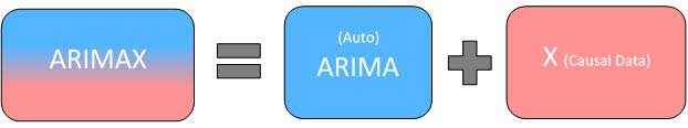
The Arimax algorithm is comparable to the Auto Arima algorithm in the way it can accommodate seasonal and non-seasonal lags, differencing (to make a time series stationary), and moving average terms without requiring that any additional parameters be specified. However, Arimax is categorized as a machine learning algorithm because it supports causal variables. The X in Arima x indicates its ability to incorporate causal data, and the linear regression equation for Arimax is expressed as:

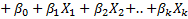
where the last k terms on the right side of the equation indicates inclusion of k causal variables.
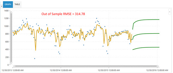
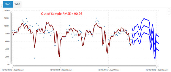
The following two graphs illustrate the effectiveness of the Arimax algorithm over the Auto Arima algorithm. Note that when appropriate causal data was available, the out-of-sample RMSE of 314.78 using Auto Arima dropped to 90.96 when using Arimax.
Auto Arima results - cannot use a causal variable -
Arimax results - can use a causal variable and increase forecasting accuracy
Because Arimax already considers lags (hence the AR in Arimax), only trend and seasonal indices are added as algorithm-generated causals.
Use this algorithm when:
- Time series length is medium to long (greater than 50 points)
- Causal data is available (Arimax can use causal data)
- For data with multiple seasonalities, Arimax performs better than Auto Arima
- Like Arima, if time series is non-stationary, Arimax algorithm can accommodate by first making it stationary
- Should not be used when number of causals is higher than number of data points in demand history
Parameters
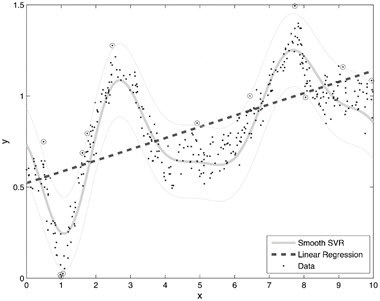
Support Vector Machine (SVM Linear)
Summary: Comparable to a non-linear regression model.
This algorithm forms a tube around the time series data by vectors (called support vectors) and evaluates the quality of the fit by a loss function (referred to as an epsilon loss function). It solves an optimization problem to determine the boundaries of this tube around the data, which minimizes the loss function.
Instead of taking scalar product of thetas and causals, the algorithm performs a “kernel trick” for non-linear regression. During this process, it combines multiple causals and fits a linear regression model of those combined causals in a higher dimension space.
The following plot shows how some non-linear patterns not captured by a linear regression model can be captured by the SVM Linear algorithm.
Use this algorithm when:
- The length of time series is long (greater than 100 points)
- Causal data is available
- Multiple user defined causal variables exist and you are using causal variables from Trend Cloud.
- Removal of outliers in the data is unnecessary; they are not considered by the algorithm while fitting to it
Parameters
- Include Causal Lags
- Demand Correlation
- Multi Collinearity Threshold
- Adjust Outliers
- Cost - if the value is too large, the algorithm attempts to fit every point, which can result overfitting. Conversely, a value that is too small can result in underfitting.
Quantile Random Forest
Summary: Build a large number of decision trees in parallel and take the average of predictions of all the trees.
Quantile Random Forest, or Random Forest (RF), is a tree-based machine learning algorithm in which approximately 500 decision trees are built. A subset of causals and a subset of data points are used to build each decision tree, and the mean of predictions from all the trees is considered as the final prediction.
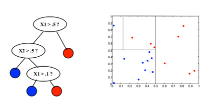
At the beginning of the algorithm, a split at the root node is made based on the most important variable (X1). This splits the data into two regions as shown to the right of the tree structure. Two new nodes are created. Assume the value X1 is greater than 0.5. On the left node at the second level, a split is made at the next-most important node (X2), which further splits the feasible region into two parts. This process is repeated until either all pre-determined variables are split, or only a small number of data points remain in the feasible region. At the last leaf node of a tree, an average of all the dependent variable values (demand points) is calculated and considered as the prediction for the next period.
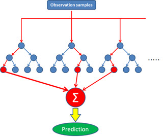
In the random forest algorithm, this procedure is repeated multiple times. Approximately 500 decision trees are built, and an average is taken of the predictions from each tree. If all the historical demand data points in the training part and all available causal variables in each tree are considered, each tree would produce the same result. Therefore, a subset of data points and a subset of causal variables are selected randomly for each tree. This method of random selection has proved effective in avoiding overfitting.
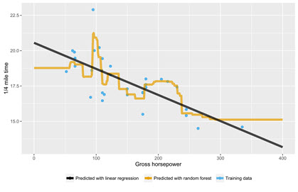
The following graph compares fitted values from a random forest algorithm to a linear regression model. Note that the random forest algorithm can accommodate more intricacies in the data, but it also tends to overfit the model. Therefore, it is important to compare in- and out-of-sample RMSE values to ensure that the algorithm is not overfitting. The two values (in and out-of-sample RMSE) should be close to each other.
Use this algorithm when:
The length of time series is long (greater than 100 points).
- Causal data is available
- Multiple user defined causal variables exist and you are using causal variables from the Trend Cloud Import action
- Always compare in- and out-of-sample RMSE values to ensure it is not overfitting
Do not use if you have an upward or downward trend in data; this algorithm cannot forecast demand values that are beyond the range of demand history (cannot extrapolate).
Parameter
- Include Causal Lags
- Demand Correlation
- Multi Collinearity Threshold
- Adjust Outliers
- No. of Randomly Selected Causal Variables - the number of causal variables randomly sampled at each node of each tree. The default value is one-third of the total number of causals used.
Model Average Neural Network
Summary: Simulates the working of the human brain.
This machine learning algorithm is inspired by the method in which biological neural networks inside the human brain process information. The basic computing unit in a neural network is called neuron/node/ unit. These nodes are connected to each other to form a neural network.

A node receives inputs from other nodes or an external source and then computes an output with an activation function inside it. This activation function is a non-linear function such as sigmoid or tanh. The activation function is needed to introduce non-linearity into the output of a neuron, because real-world data is often non-linear and the neurons must learn these non-linear relationships.
The neural network shown in the bottom right section of the previous example is a Feedforward neural network. This network type includes three types of layers:
- input, of which there can be more than one
- hidden, of which there can be more than one
- output, of which there is typically one
In a Feedforward neural network, the information moves in one direction - from the input to the output layer.
The internal algorithm used for training a Feedforward neural network is referred to as the backpropagation algorithm. The connection between nodes of adjacent layers have weights associated with them, and the learning goal (training) in this case is to estimate the correct weights of these connections. Once all the weights are learned correctly, the trained neural network can be used to make predictions for future demand.
Use this algorithm when:
- At least 100-150 data points are available; less data points can result in overfitting
- Multiple user defined causal variables exist and you are using causal variables from the Trend Cloud Import action
- Always compare out-of-sample RMSE with a simple classic algorithm to check performance
Parameters
- Include Causal Lags
- Demand Correlation
- Multi Collinearity Threshold
- Adjust Outliers
- No. of Hidden Units - number of nodes/units in the hidden layer. The default value is optimized by the algorithm.
- Weight Decay - value for weight decay to help avoid overfitting. The default value is optimized by the algorithm.
- Bagging - if set to TRUE, each repeat of a neural network trains on a sample of the training data. The default value is FALSE.
Stochastic Gradient Boosting
Summary: Use Stochastic Gradient Boosting to build a large number of decision trees sequentially, and keep improving the model iteratively by building more trees.
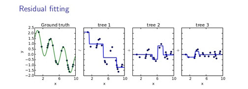
Gradient Boosting Machine (GBM) is another decision tree-based algorithm. It is iteration-based and uses residual fitting to minimize a loss function. Initially, a decision tree model is created (tree 1) to fit to the original data, and residuals are calculated from the fit. Then, another tree (tree 2) is built that fits to the residuals, and the residuals are calculated between the fit of tree 2 and the residuals from the initial fit, and another decision tree model (tree 3) is fit on that. In this manner, the decision trees are created sequentially, and the predictions of all the trees are added together to form the final prediction. Care is taken to not overfit to the data.
Use this algorithm when:
- The length of time series is long (greater than 100 points)
- Causal data is available
- Multiple user defined causal variables exist and you are using causal variables from the Trend Cloud Import action
- Always compare in- and out-of-sample RMSE values to ensure it is not overfitting
Do not use if you have an upward or downward trend in data; this algorithm cannot forecast demand values that are beyond the range of demand history (cannot extrapolate).
Parameters
- Include Causal Lags
- Demand Correlation
- Multi Collinearity Threshold
- Adjust Outliers
- No. of Boosting Operations - the total number of trees to fit. Equivalent to the number of iterations.
- No. of Splits - the number of splits performed on a tree.
- Shrinkage - the learning rate or step-size reduction. Applied to each tree.
- Min. Terminal Node Size - minimum number of observations in the trees’ terminal nodes.
Last modified: Thursday December 19, 2024