Classic algorithms
Classic algorithms are generally used when no causal data is available, the time series is short (not many data points), and the behavior of time series is random (less patterns in data). Note that these are general criteria; some classic algorithms work well even for long time series and time series involving clear seasonal patterns.
Characteristic of classic algorithms include:
- Cannot work with causal data
- Generally used when the time series length is small to medium (10 – 50)
- Naïve and Simple Moving Average algorithms best used for benchmarking results
- If time series is non-stationary, Arima or Auto Arima algorithm should be used
Naïve Forecasting
Summary: Previous value is the next prediction
Naïve forecasting is the simplest type of time series forecasting algorithm. It chooses the most recent value as the next prediction. Using our ice cream sales example, if yesterday’s ice cream sale was $960, the Naïve forecasting algorithm will predict today’s ice cream sale as $960. This algorithm is used when the time series data is quite random and does not include any seasonality or other clear patterns; in other words, the forecastability of the time series is low.
Forecastability of a time series refers to the ease with which its future values can be predicted. If you toss a coin and assign 1 for heads and 0 for tails, then a sequence of tosses will generate a time series with values 0 and 1. If the coin is fair, then this will be a random sequence and the forecastability of the realized time series will be very high (extremely difficult to forecast). On the other hand, if a time series is following a clear sinusoidal pattern, then it would be much easier to predict its future values. In cases where the forecastability of a time series is low, use of Naïve forecasting should be avoided.
Use this algorithm when:
- You have a very small number of data points in your time series (more sophisticated algorithms won’t perform well).
- Your data is relatively random, no clear seasonality or trend exists, and the forecastability is high (difficult to forecast).
- Generally used for benchmarking purposes. It helps you to understand how well a sophisticated forecasting algorithm is performing when compared to Naïve forecasting.
Example
Parameters
Simple Moving Average
Summary: Take the average of past k values
Simple Moving Average is the unweighted mean of the last k observations in a time series, where k is a parameter. So, the prediction at time t, xt is expressed as:
In the ice cream sales example, if k = 7, then the sale prediction for the next day would be (880 + 920 + 900 + 910 + 930 + 950 + 960) / 7 = $921.4. But if k = 4, our prediction would be (910 + 930 + 950 + 960) / 4 = $937.5. So, how do you decide what value of k to use? And when should you use simple moving average as a forecasting algorithm?
The value of k depends on the data. If more recent values are affecting the current demand, then the value of k should be small. But if the data is fluctuating more, it is better to have larger value of k.
Use this algorithm when the current demand value is dependent on the last few data points and:
- Clear seasonality does not exist.
- Fewer data points are available in time series.
- For benchmarking purposes
- The data is less forecastable (high forecastability index value).
Example
Parameters
- Include Causal Lags
- Demand Correlation Threshold
- Multi Collinearity Threshold
- Adjust Outliers
- - the number of immediate past observations to be included in the simple moving average (k). The default value is Auto, which means the algorithm optimizes this parameter internally and yields the best value of Moving Average Type based on some testing (currently it chooses between values between 2-20).
-
- by default, is set to FALSE. When set to TRUE, then instead of taking the simple moving average of last k observations, this parameter determines the center value of the time series (by time) and calculates the symmetric mean of an approximately equal number of demand points on either side of the center value, including the center value itself. For example, if there are 15 data points in the time series and k = 5, then the next prediction is the average of the 6th, 7th, 8th, 9th and 10th data points (as shown in orange):


Exponential Smoothing
Summary: Take the weighted average of past observations. The weights decrease exponentially.
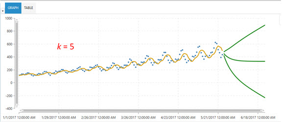
Instead of giving equal weight to the previous data points, exponential smoothing gives the highest weight to most recent demand point and progressively less weight going further back in the demand history. The result is a weighted mean of the historical demand with weights decreasing exponentially.
Use this algorithm when:
- The length of the time series is short to medium (20 to 50 points). It can work well on longer time series too.
- Your data has seasonality and/or a trend.
- Causal data is not available.
- If the slope of the trend is changing, an exponential smoothing algorithm can pick it up quickly.
Example
Let xt+1 be the demand at time t+1. Let st be the prediction given by the Exponential Smoothing algorithm based on the past t data points in a time series. According to exponential smoothing:
In this equation,  is called as a smoothing parameter to determine how the weight should be distributed among the historical data points while calculating the weighted mean. If
  in the previous equation, that means 60% weight is assigned to the last data point
  and the balance of 40% weight is assigned to the remaining data points in the demand history. But, how does exponential smoothing distribute the remaining 40% weight to the remaining data points?
Expanding the previous equation results in:


Note that the weight assigned to  is
is  , the weight assigned to
  is
is  , and then for
  is
is  . If
. If  , the weights are 0.4, 0.24 and 0.144 respectively. If the equation is expanded even further, the weights are:

Not only are the weights decreasing for older data points, but they are decreasing in an exponential manner.
The algorithm just described is simple exponential smoothing. Apart from past values, the Exponential Smoothing algorithm can also capture trend and seasonality in the data.
Trend represents a long-term progression of the data. If the data has a directionality (increasing or decreasing), it is because of this trend component. Trend can be linear or non-linear. Seasonality is simply repetitive seasonal variations in the data. Increasing ice cream sales on the weekends, or increasing merchandise and electronic devises sales during Christmas, are some examples of seasonal fluctuations. Seasonality can be weekly, monthly, quarterly, or annual; it can also have any non-standard period, such as repeating after a specific number of weeks.
An exponential smoothing algorithm that considers past values and trend is referred to as a double exponential smoothing algorithm, while one that considers all three components (past values, trend, and seasonality) is a triple exponential smoothing algorithm.
Parameters
- Include Causal Lags
- Demand Correlation
- Multi Collinearity Threshold
- Adjust Outliers
- Seasonal Frequency
The parameters are estimated by the algorithm automatically. If neither trend nor seasonality exist in the data, then the values of  and
and  will be zero. In that case, the algorithm becomes simple exponential smoothing.
Use Seasonal Frequency to control the period of the data. If you know that the data repeats every year, and if it is weekly data, then the value of seasonal frequency would be 52 (there are 52 weeks in a year). The default value of this parameter is set to Auto, meaning the algorithm optimizes the seasonal frequency value if it is unknown.
Arima
Summary: A linear regression model of lags and moving average terms. Differencing is performed to make the time series stationary.

Arima (AutoRegressive Integrated Moving Average) is a linear regression of lags (AR part) and moving average (MA part).
A time series is said to be stationary when its mean, variance, and autocorrelation (lags) structure do not change over time. For example, if an upward trend exists in the data, it becomes a non-stationary time series.
If a time series is non-stationary, the Arima algorithm will take difference(s) between consecutive values of the time series to make a new time series. Taking such differences will make a time series stationary. This differencing is the I part in ARIMA.
To understand Arima, you must first understand what linear regression is. Linear regression is an approach that models the relationship between a dependent variable Y and one or more independent variable(s) X.
In its simplest form, this can be represented as:

Use this algorithm when:
- The length of time series is short to medium (20 to 50 points). It can work well on longer time series too.
- If your data has seasonality and a trend, the Arima algorithm can use them to make better predictions.
- Causal data is not available.
- If your time-series is non-stationary, the Arima algorithm can make it stationary.
- If an older lag (lag 5) is more important than a newer lag (lag 3), then Arima can assign appropriate weights. Exponential smoothing cannot do this; it will always assign a higher weight to lag 3 than to lag 5.
Example
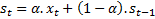
Using the ice cream sales example, X is an independent variable such as temperature, and Y is the dependent variable such as ice cream sales. If we plot values of temperature and ice cream sales from the example, with temperature on X axis and ice cream sales on Y axis, the plot looks like the following:
In this plot, the blue dots represent the true data, and the red line represents a line that best fits the data. The equation of the line is Y = -280.71 + 15.95*X, meaning that the estimated value of  is -280.71, while that of
  is 15.95. This (toy) example had only one independent variable X. In general, this can be expressed as:

Lags are simply historical demand values. Lag 1 represents demand value in the previous period, Lag 2 represents demand value two periods ago, and so on. Therefore, if we are dealing with daily data, Lag 1 is yesterday’s demand, but if we are dealing with weekly data, then Lag 1 represents demand occurred last week.
Moving average (model) is not the same as simple moving average. Moving average is the error values between actual data and fitted values. For example, in the plot shown in Naïve Forecasting, the regression line does not pass through all the data points. When the temperature was 72F, the actual ice cream sale was $880, but the fitted value (point on the regression line) was $867.9. Therefore, the error term is (880 - 867.9 = 12.1). The moving average model is regression of such error terms in from the demand history.
After making a time series stationary, the Arima algorithm builds a linear regression model of lags and moving average terms. Thus, demand in period t is modeled as:

Here,  to
to  are the first p lags and
  and
and  are the first q moving average terms. The alphas are coefficients of lags and the thetas as coefficients of moving average terms.
Notes
The Arima algorithm can also accommodate seasonal lags, seasonal differencing, and seasonal moving average terms. For example, if your data is weekly and it has annual seasonality, the seasonal lag 1 indicates the demand value occurred in the same week of the previous year. Similarly, seasonal moving average term 1 indicates the error between the demand that occurred in the same week of the last year and the corresponding fitted value.
Parameters
- Include Causal Lags
- Demand Correlation
- Multi Collinearity Threshold
- Adjust Outliers
- Non-seasonal Auto-Regressive Lag - auto-regressive order (number of lags)
- Non-seasonal Difference - difference order (number of times the differences were taken to make the time series stationary)
- Non-seasonal Moving Average Lag - moving average order (number of error terms)
- Seasonal Auto Regressive Lag - seasonal auto-regressive order (number of seasonal lags)
- Seasonal Difference - seasonal difference order (number of times the differences were taken across the season to make the time series stationary)
- Seasonal Moving Average Lag - seasonal moving average order (number of seasonal error terms)
- Seasonal Frequency - number of periods after which the pattern in the data is repeating
Auto Arima
Summary: Conceptually the same as that of Arima algorithm; however, parameters are selected automatically by the algorithm.
The best values for all the parameters in the model are determined automatically according to the following, which are listed in order of priority:
- AICc (Corrected Akaike Information Criterion)
- AIC (Akaike Information Criterion)
- BIC (Bayesian Information Criteria)
The method conducts a search over all possible parameter values within the constraints.
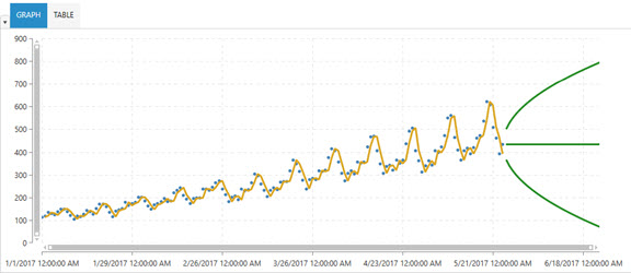
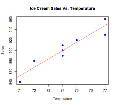
Use of the wrong parameter values can yield incorrect results. For example, the following is an example of an Arima algorithm using parameters (p,d,q) (P,D,Q) [seasonalFrequency] selected as (0, 0, 1) (0, 0 , 0) [1].
The blue dots indicate the actual data. Note that neither the fit (yellow line), nor the predictions (center green line) are a good fit. The out of sample RMSE (forecast error on test sample) is 215.2.
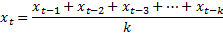
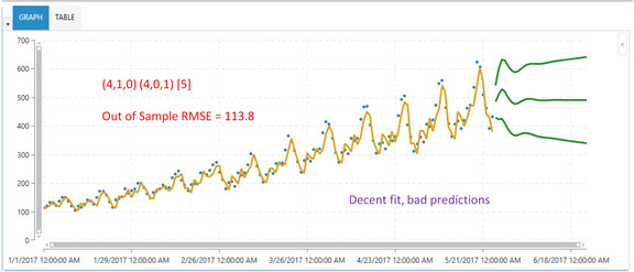
The following shows a better choice of Arima parameters. The parameter values are (4, 1, 0) (4, 0, 1) [15]. While the model fit is good, the predictions are still not capturing the pattern in the data. The out of sample RMSE value is now reduced to 113.8.
However, using the Auto Arima algorithm to choose the parameters can lead to much better results, as shown in the following:
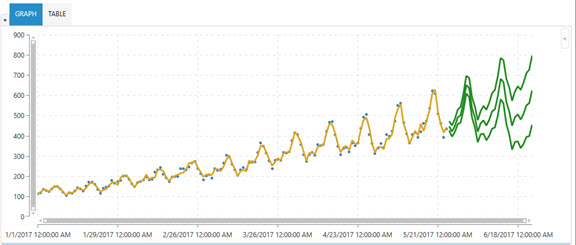
Note that the fit is good and the predictions seem to be much more accurate, while the out of sample RMSE is reduced to 26.99.
When to use?
- The length of the time series is short to medium (20 to 50 points), although it can work well on longer time series too.
- If the data has seasonality and a trend, the Auto Arima algorithm can use them to make better predictions.
- Causal data is not available.
- If your time-series is non-stationary, the Auto Arima algorithm can handle it by first making it stationary.
- If an older lag (such as 5) is more important than a newer lag (such as 3), then the Auto Arima algorithm can assign appropriate weights. Exponential smoothing cannot do this; it will always assign a higher weight to lag 3 than to lag 5.
Parameters
Parmeters are the same as those used in the Arima algorithm:
- Include Causal Lags
- Demand Correlation
- Multi Collinearity Threshold
- Adjust Outliers
- Non-seasonal Auto-Regressive Lag - upper bound of 5
- Non-seasonal Difference - upper bound of 2
- Non-seasonal Moving Average Lag - upper bound of 5
- Seasonal Auto Regressive Lag - upper bound of 2
- Seasonal Difference - upper bound of 2
- Seasonal Moving Average Lag - upper bound of 2
- Seasonal Frequency - number of periods per season, which is the number of periods after which the pattern in the data is repeating. This is an optional parameter. If you do not provide its value, the algorithm finds the best possible value.
Last modified: Thursday December 19, 2024