Piecewise-linear life cycle models

A traditional product life cycle typically includes the following stages:

• Launch
• Growth
• Maturity
• Decline
• Obsolescence

Non-linear life cycle algorithms (for example, the Logistic alogrithm) can capture this type of full life cycle. However, some products may have already existed in the market under a different version. For example, consider the original version of a laptop computer. Each new version of that laptop can be regarded as a new product, even though it is only an extension of the existing product (the original laptop computer) in the market. Life cycles of new product versions may deviate from commonly known product life cycles. This phenomenon occurs especially during the launch, obsolescence, and maturity stages.

• New version sales may start immediately with a growth stage, since the product line is already well-known by the market. If sales start to increase as soon as the new version is introduced in the market, there is no launch stage.
• The new version can affect the maturity stage of the previous version, and the existing version may not actually have any maturity stage.
• The new version can cease to exist abruptly during decline stage due to the introduction of another new version. For such versions, the growth stage is immediately followed by a decline stage, and the product ceases to exist in the market without exhibiting any obsolescence stage.

Demand Guru provides two algorithms to model this behavior: Triangle and Trapezoid. These algorithms are referred to as piecewise-linear, because they are composed of two or three linear regression lines. They are relatively simple when compared to non-linear life cycle algorithms. Not only are these algorithms easy to comprehend, but they are also easy to quantify because you can provide practical input parameters, such as total life time.

Non-linear life cycle algorithms are fitted to S-shape cumulative demand data, and then fitted demand values are extracted from the cumulative fit. However, piecewise-linear life cycle algorithms are fitted directly to the demand data. Cumulative values of these fitted demand values will also form an S-shape cumulative demand curve.

Triangle life cycle algorithm

The Triangle algorithm consists of two stages: Growth and Decline.

Parameters include:

• Product Life - Total life of the product.
• Half Life - Total duration of time from the start to the end of the growth stage. This is when product sales are increasing. At the end of this stage, sales are at peak level. After this stage, the product enters the decline stage.
• Growth Slope - The rate at which a product rises to peak level sales, which can be quantified as the demand at the end of half-life over half-life.
• Decline Slope: The rate at which a product's demand declines, which can be quantified as the demand at the peak level over the total time that the product is in the decline stage.

A typical Triangle Life Cycle Fit is shown in the following plot:

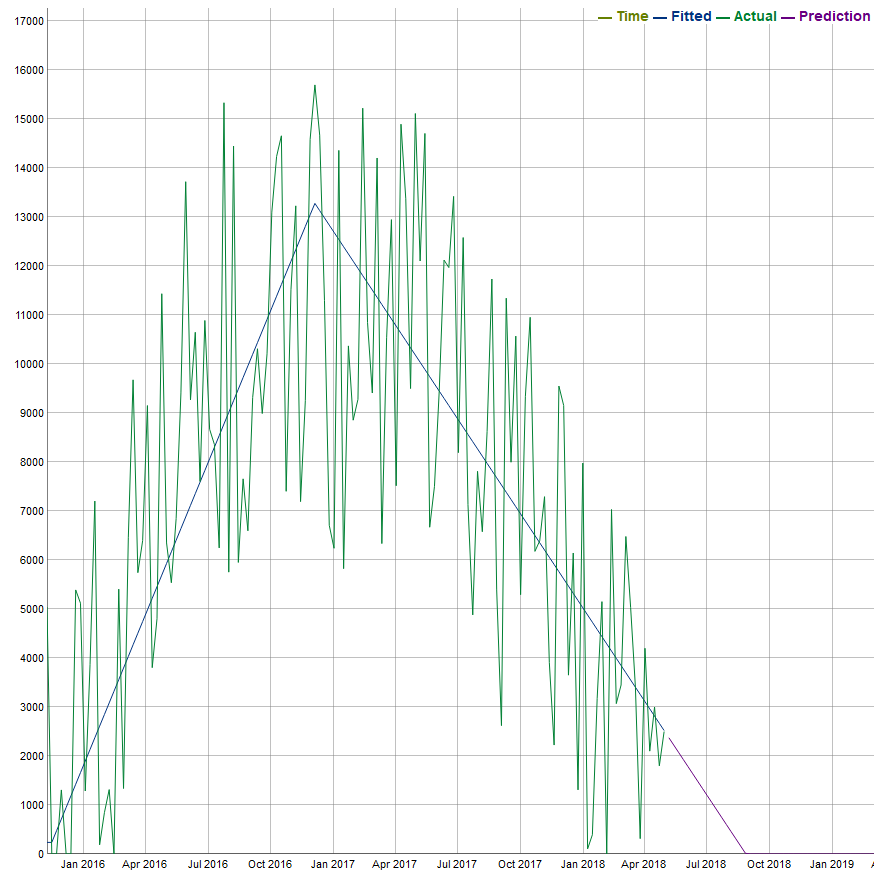
The Triangle algorithm includes two piecewise linear lines:

• The first line models the growth stage.
• The second line models the decline stage.

Calculations are based on the following:

In this plot, time duration a represents half-life and growth stage length, while time duration c represents decline stage duration. Product life can be estimated as a+c. The demand at the end of half-life (peak demand) is represented by b. In this case, growth slope is defined as b/a, while decline slope is defined as -b/c.

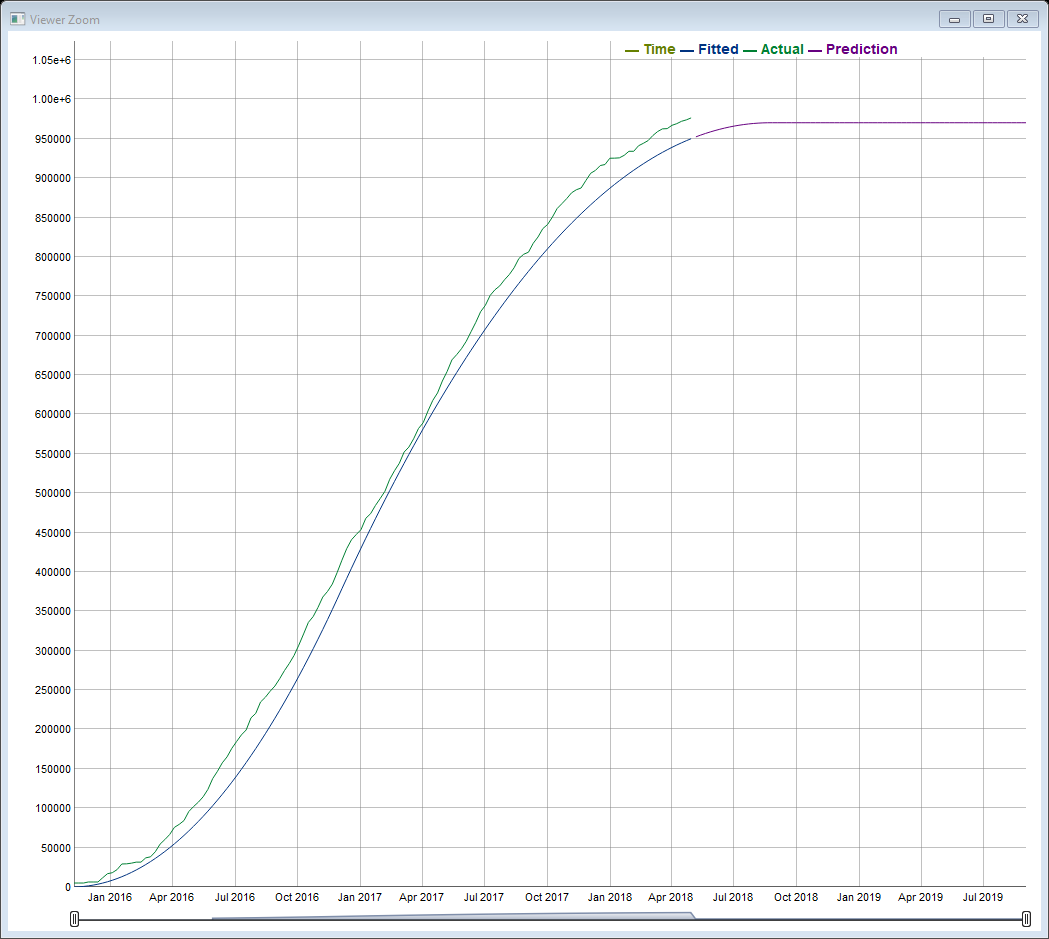
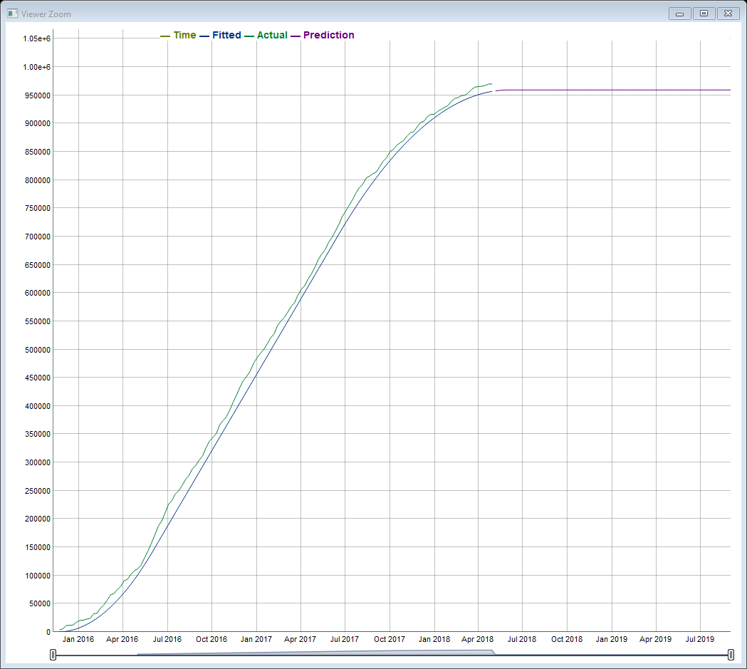
As shown by the fitted lines, the life cycle does not have a launch, maturity, or obsolescence stage. However, this algorithm clearly captures both the growth and decline trends. After fitted demand values are generated by the algorithm, a cumulative S-shape curve is generated:

Trapezoid life cycle algorithm

The Triangle algorithm consists of three stages: Growth, Maturity and Decline. The maturity stage is represented by a flat line.

Parameters include:

• Product Life - Total life of the product.
• Maturity Point - Total duration of time from the start to the end of the growth stage. This is when product sales are increasing. At the end of this period, the maturity stage begins.
• Declination Point - Total duration of time from the start of the growth stage to the end of the maturity stage. At the end of this period, the product enters the decline stage.
• Growth Slope - Defines the rate at which a product rises to maturity.
• Decline Slope - Defines the rate at which a product's demand declines.

A typical Trapezoid Life Cycle Fit is shown in the following plot:

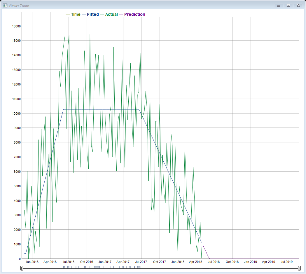
The Trapezoid Life Cycle algorithm has three piecewise linear lines:

• The first line models the growth stage.
• The second line is a flat line used to represent the maturity stage.
• The third line models the decline stage.

As shown by the fitted lines, the life cycle does not have a launch or obsolescence stage. However, this algorithm clearly captures the growth, maturity, and decline trends.

Calculations are based on the following:

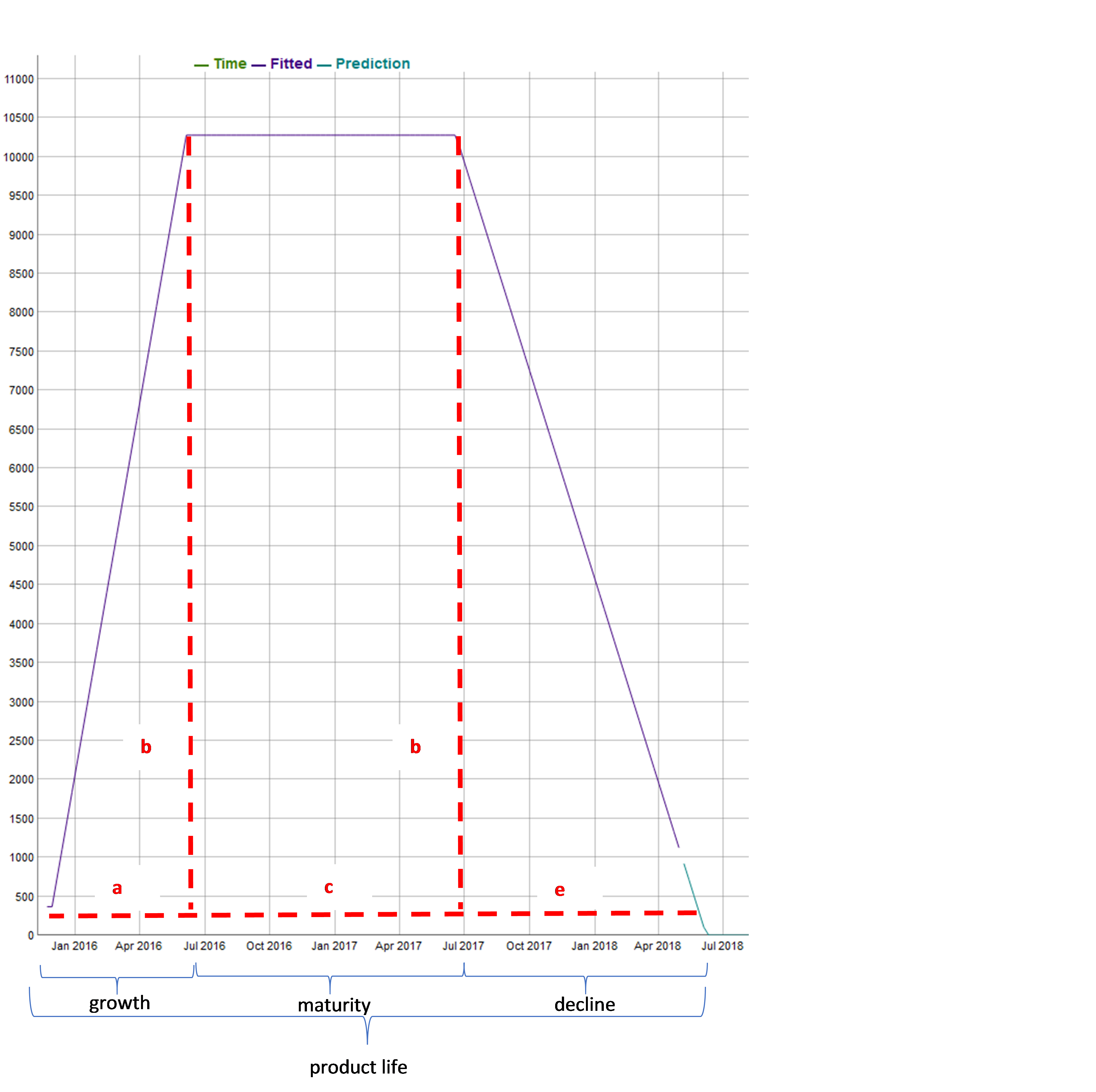
In this plot, time duration a represents half-life and growth stage length, time duration c represents maturity stage duration, and time duration e represents decline stage duration. Product life can be estimated as a+c+e. Peak demand is represented by b. In this case, growth slope is defined as b/a while decline slope is defined as -b/e.

After fitted demand values are generated by the algorithm, a cumulative S-shape curve is generated: