Feature extractions for clustering

Time series each exhibit certain characteristics. During the clustering process, Demand Guru extracts 16 such characteristics from each time series, and these characteristics are the features that form the basis of clustering.

For example, mean is a feature that refers to the mean demand value of a time series. Time series with mean demand values that are close to each other share a similarity, and so time series can be grouped into clusters based on similar mean values.

The shapes of these time series can be totally different, and their mean values cannot capture shapes. However, mean is just 1 of 16 features.

Other features can be used to capture additional similarities between time series: Seasonality is another feature, and time series having the same seasonality period are said to be similar with respect to that feature. Trend is also a feature, and if two time-series are trending upward with similar slope (similar trends), they are said to be similar with respect to that feature.

When you extract a feature from a time series, you are actually calculating a score and assigning it to that feature. The distance between feature scores allows you to calculate similarity between time series, which in turn helps to form clusters. If you extract k features, then the Euclidian distance calculated across those k features provides a distance between all the time series.

The following features can be extracted:

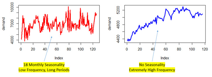
Seasonality

A coefficient value based on the periodicity of the most prominent seasonal period in a time series. Low values indicate low frequency or long period seasons, while high values indicate high frequency or short periodic time series. An absence of seasonality in the data is assumed to indicate extremely high frequency (noisy data) and has a high value associated with it.

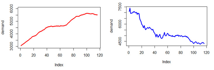
Trend

An index of the strength of a trend. High positive values indicate strong upward trend, high negative values indicate a strong downward trend, and values close to zero indicate that the trend is flat. In the following example, the graph on the left shows a trend coefficient score of 0.328, while the graph on the right shows a trend coefficient score of -0.287.

Mean

Mean of the demand values in a time series.

Variance

Variance of the demand values in a time series.

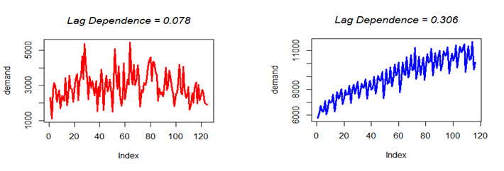
Auto Correlation

Represents the extent of dependence on past demand values. While calculating this score, 10 lags are considered. A higher dependence of the time series on its past 10 values results in a higher auto correlation score.

Lumpiness

The variability of variance of each period in a time series. Conceptually, divide the time series into multiple sections, calculate the variance of each section, and then calculate the variance of these variance values. Low values indicate that the variance of the time series does not change much across its different sections, while high values indicate the variance is changing a lot across different sections of a time series.

Level Shift

The maximum absolute value of mean values of slices of a time series, when a rolling window (of size =1) is used. Seasonal time series are divided into multiple slices, with the slice length equal to its most prominent period. For non-seasonal time series, this slice length is equal to a fixed constant.

The first slice is rolled by the window size (= 1 here), and the maximum absolute value of the mean of the rolled slice gives the value of the level shift.

Intuitively, this value represents the maximum “level” in a section of a time series.

Variance Change

The maximum absolute value of variance values of slices of a time series, when a rolling window (of size =1) is used. Seasonal time series are divided into multiple slices, with the slice length equal to its most prominent period. For non-seasonal time series, this slice length is equal to a fixed constant.

The first slice is rolled by the window size (= 1 here), and the maximum absolute value of the variance of the rolled slice gives the value of the variance change.

Intuitively, this value represents the maximum variance in a section of a time series.

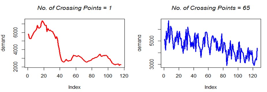
Crossing Points

The number of times a time series crosses the midpoint of its range. Range is nothing but (Maximum value – Minimum value). In the following example, the graph on the left shows a time series that crosses the midpoint of its range just a single time, while the time series in the graph on the right crosses the midpoint of its range 65 times.

Linearity

Strength of the linearity component of a time series, with high values indicating strong linearity, and positive values indicating an upward trending time series.

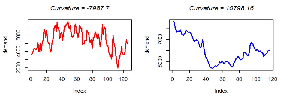
Curvature

The strength of a trend's curvature component in a time series. Positive values indicate convex shaped time series, while negative values indicate concave shaped time series.

Peak

Strength of the highest point on the seasonal component of a time series.

Trough

Value of the lowest point on the seasonal component of a time series.

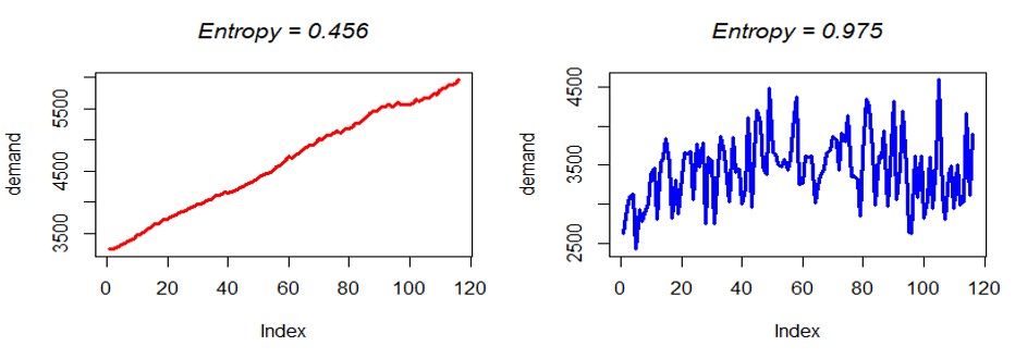
Entropy

A measure of the forecastability of a time series. It reveals the degree of difficulty associated with forecasting a specific time series, based on only the demand values. Low values indicate that the time series is relatively easy to forecast, and higher values indicate increased difficulty.

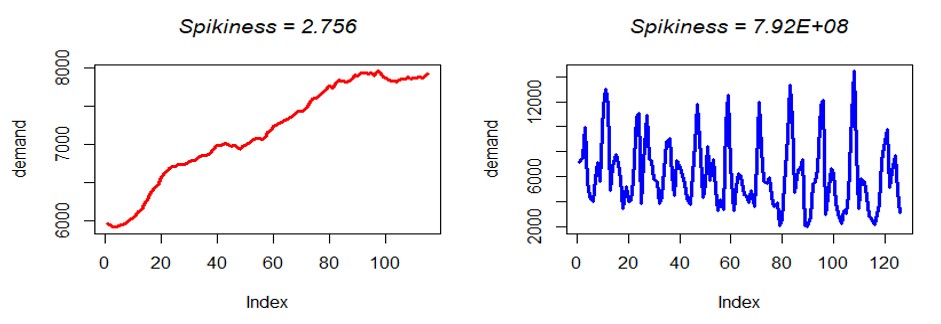
Spikiness

The strength of spikes of residuals in a time series. The seasonality and trend components are first removed, and then the value is calculated over the residual component.

Flat Spots

The length of flat spots in a time series. To arrive at this value, a time series is broken down into multiple discrete levels. Then, an analysis is made to determine the number periods for which the time series maintains the same level. The overall length of these periods provides the value for this feature.

In the following example, the graph on the left shows a time series with a flat spot value of 2, which means the time series is changing its discretized levels quite often. Conversely, the graph on the right shows a time series with a flat spot value of 69, meaningthe time series is staying in the same level for 69 consecutive periods.