Effect of algorithms on life cycle curve

Let t be the time points for which the function values will be returned. The function y(t) shows the total cumulative demands; that is, the function calculates the values of the growth curve for given time points. The S-shaped curve can be represented as shown in the following graph with the foregoing parameter characterization.

• - Maximum of the curve. This parameter controls the maximum cumulative growth, which is a measure of the upper limit of market sales or the total market capacity.
• - Maximum slope. This parameter controls how quickly a product reaches out to its end-life or how quickly a product diffuses into a market.
• - Lag-phase. This parameter controls how long the initial (born) stage takes.

Each Life Cycle treats these parameters differently, as shown in the following equations.

Logistic Growth Model

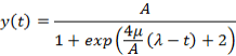
where refers to .

Richards Growth Model

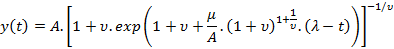
where refers to an additional shape parameter.

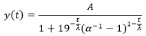
Gompertz Growth Model

For a given data set, these three models’ parameters are estimated using R function nls(…). Depending on the data, fitting may or may not be successful. In case of unsuccessful data sets, we recommend that the modeler should increase the size of the data.

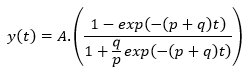
Modified Logistic Growth Model (Yelland 2004)

where and is the initial data value.

Monomolecular Model (France et al. 1996)

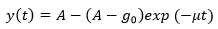
Note that both the modified logistic and monomolecular models have the initial value as a common input parameter. However, these two models use different parameters: the modified logistic model uses lag phase , while the monomolecular model uses maximum slope in addition to max growth and initial value parameters.

Bass Growth Model (Bass 1969)

where is the effect of innovators (buying the product using information about the product, advertisements, and so on), and is the effect of imitators (buying the product based on the experiences of other people, their ratings, word of mouth, and so on).

The Bass modeling approach is different than previously discussed models - it captures the cumulative sum of demand gained through the effects of innovators and imitators.

The previous plots indicate that the total cumulative sales (growth) is created by two types of demand:

• product sales starting with the effect of innovators
• product sales starting later with the effect of imitators

Note that cumulative sales (growth) follows an S-shaped curve.

For a given data set, the parameters are estimated by using the R function nls(…) for the nonlinear least number of squares fitting of these models. Depending on the data, fitting may or may not be successful. For unsuccessful data sets, we recommend that you increase the size of the data.

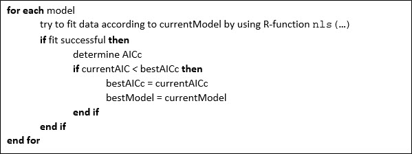
Tournament Life Cycle Model

The tournament model runs all the available life cycle models and chooses the best model based on the selected model criteria:

• AIC (Akaike Information Criterion with correction)
• AICc (Akaike Information Criterion with correction)
• BIC (Bayesian Information Criterion) and Cross Validation (RMSE – out of sample root mean square estimate)

The default criteria is AICc. The algorithm that provides the lowest AICc value over the fit period is selected as the best algorithm. The underlying algorithm is given as: