Analyze a transaction table

In Data Guru, a variety of different actions are available for analyzing data to assist you in decision making. Each action offers advantages that depend on the nature of the data and the analysis being performed.

This example analyzes a transactions table. The analysis looks at the integrity, accuracy, and variance of the data, along with order variation patterns, and creates a "boxplot" for further visualization and analysis. The following analysis actions are featured:

• Data Profiling
• Demand Analysis
• R Scripting

The data in this example is made available using a delimited file connection using a CSV file called TransactionalData. This file contains some sample customer transactions that you will import to a new table named ShipmentTransaction. The new table contains information that includes:

• Category information (fields Category_ID and Item_Category)
• Department information (fields Department_ID and Dept_Description)
• Sub-Department information
• Item information (fields Item_Number and Item_Descr)
• Shipping information (fields Shipping_DC, Destination_ID, and Customer_Store)
• Shipped quantity (field name is Ship_Qty)
• Ship date (field name is Ship_Date)

Initial Setup:

1. Create a new Data Guru project.

2. Add a New Delimited File Connection.

   • Select the TransactionalData.csv file that you downloaded.

   • Click Edit Mapping and ensure that the "First row contains column names" option is selected.

3. Create a macro, then add a Delimited File Import action.

   • The Delimited File Connection is "TransactionalData"

   • The Table Name in Output is "ShipmentTransaction".

4. Run the action to import the data into the new ShipmentTransaction table.

Once the table is imported, you can analyze and manipulate the data.

Step 1 - Use Data Profiling to analyze the transaction data.

1. Select ShipmentTransaction as the input table. Output tables will be ShipmentTransaction_TS and ShipmentTransaction_CV.
2. On the Configuration tab, click >> to select all the fields. This will analyze the entire table. The fields are analyzed differently based on their data type. Since there are database constraints for what can be stored in numeric and date fields, Data Profiling provides more insight into the contents of text fields such as Item_Descr and Shipping_DC.
3. Upon completion of the action, open the ShipmentTransaction_TS table to view the profiling. The results show that several columns have blank values. These rows must be removed.

Step 2 - Use the Data Fork action to remove the incomplete rows.

1. Select ShipmentTransaction as the input table.
2. Specify Demand as the match table and FailTransactionData as the non-match table.
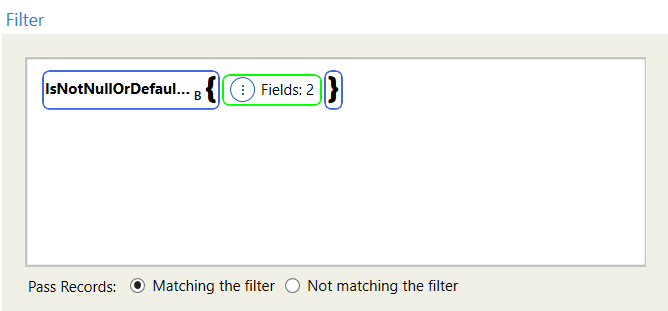
3. Use the IsNotNullOrDefaultAll function on fields Item_Descr and Shipping_DC and select the Matching the filter option. Only those records that match the filter will be passed, filtering out those columns that have a blank or null value.
   

Step 3 - Use the Demand Analysis action to analyze the Demand table, which has invalid entries removed.

1. Specify Demand as the input table, and DemandClassification as the output table.
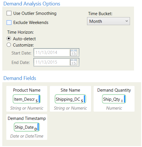
2. Map the field names into the input fields and set the Time Bucket to Month.
   
3. The resulting DemandClassification table displays the demand characteristics and statistics for each site-product combination, along with the associated classifications. Data Guru classifies your demand based upon intermittency, variability, demand class, and clumpiness.

Step 4 - Use the Create Table transform to create a new table with the appropriate structure.

1. Specify Shipment_Frequency as the output table.
2. Specify the following columns for the new table:
   • Sub_Dept_Descr with a type of StringU (255)
   • Customer_Class with a type of StringU (255)
   • Frequency with a type of Double

Step 5 - Use the R Scripting transform to output a data frame to the new Shipment_Frequency table.

1. Specify the Demand table as the input table, and Shipment_Frequency as the output table. Both tables will be treated as data frames by R Script.
2. On the configuration tab, specify the R script as follows:
   
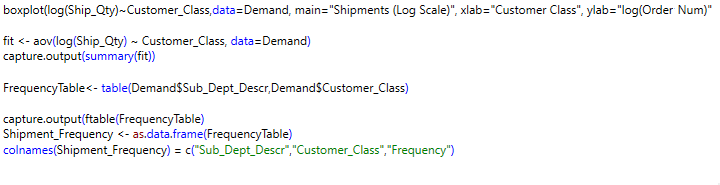
3. In the R Script, a boxplot is being created that plots the Log of the shipped quantity for each customer class. An analysis of variance is being performed on the same relationship. Capture.output is used to display the summary of that analysis in the html output of the action. The number of occurrences of each sub-department description, customer class combination is counted, and Shipment_Frequency is defined as a data frame containing these results, with the same column structure as the Shipment_Frequency output table.
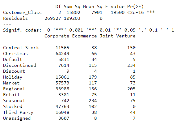
4. Analyze the Shipment_Frequency table. You also can view the boxplot results in html format, which can be launched from the radial menu. Below the boxplot, you can view the text summary and matrix that were written to this html output using capture.output.